Chapter 2 Reading in Spatial Data

There are several ways we typically get spatial data into R:
- Load spatial files we have on our machine or from remote source
- Load spatial data that is part of an R package
- Grab data using API (often making use of particular R packages)
- Converting flat files with x,y data to spatial data
- Geocoding data (we saw example of this at beginning)

For reading and writing vector and raster data in R, the three primary packages you’ll use are:

sf or rgdal for vector formats such as ESRI Shapefiles, GeoJSON, and GPX - both packages use OGR, which is a library under the GDAL source tree,under the hood
raster for raster formats such as GeoTIFF or ESRI or ASCII grid using GDAL under the hood

We can quickly discover supported I/O vector formats either via sf or rgdal:

library(knitr)
library(sf)
library(rgdal)
print(paste0('There are ',st_drivers("vector") %>% nrow(), ' vector drivers available using st_read or read_sf'))

## [1] "There are 82 vector drivers available using st_read or read_sf"

kable(head(ogrDrivers(),n=5))

name	long_name	write	copy	isVector
AeronavFAA	Aeronav FAA	FALSE	FALSE	TRUE
AmigoCloud	AmigoCloud	TRUE	FALSE	TRUE
ARCGEN	Arc/Info Generate	FALSE	FALSE	TRUE
AVCBin	Arc/Info Binary Coverage	FALSE	FALSE	TRUE
AVCE00	Arc/Info E00 (ASCII) Coverage	FALSE	FALSE	TRUE

kable(head(st_drivers(what='vector'),n=5))

	name	long_name	write	copy	is_raster	is_vector	vsi
PCIDSK	PCIDSK	PCIDSK Database File	TRUE	FALSE	TRUE	TRUE	TRUE
netCDF	netCDF	Network Common Data Format	TRUE	TRUE	TRUE	TRUE	FALSE
PDS4	PDS4	NASA Planetary Data System 4	TRUE	TRUE	TRUE	TRUE	TRUE
JP2OpenJPEG	JP2OpenJPEG	JPEG-2000 driver based on OpenJPEG library	FALSE	TRUE	TRUE	TRUE	TRUE
JPEG2000	JPEG2000	JPEG-2000 part 1 (ISO/IEC 15444-1), based on Jasper library	FALSE	TRUE	TRUE	TRUE	TRUE

As well as I/O raster formats via sf:

library(knitr)
print(paste0('There are ',st_drivers(what='raster') %>% nrow(), ' raster drivers available'))

## [1] "There are 144 raster drivers available"

kable(head(st_drivers(what='raster'),n=5))

	name	long_name	write	copy	is_raster	is_vector	vsi
VRT	VRT	Virtual Raster	TRUE	TRUE	TRUE	FALSE	TRUE
DERIVED	DERIVED	Derived datasets using VRT pixel functions	FALSE	FALSE	TRUE	FALSE	FALSE
GTiff	GTiff	GeoTIFF	TRUE	TRUE	TRUE	FALSE	TRUE
NITF	NITF	National Imagery Transmission Format	TRUE	TRUE	TRUE	FALSE	TRUE
RPFTOC	RPFTOC	Raster Product Format TOC format	FALSE	FALSE	TRUE	FALSE	TRUE

2.1 Reading in vector data

sf can be used to read numerous file types:

Shapefiles
Geodatabases
Geopackages
Geojson
Spatial database files

2.1.1 Shapefiles

Typically working with vector GIS data we work with ESRI shapefiles or geodatabases - here we have an example of how one would read in a shapefile using sf:

# download.file("ftp://ftp.gis.oregon.gov/adminbound/citylim_2017.zip","citylim_2017.zip")
# unzip("citylim_2017.zip", exdir = ".")
library(sf)
citylims <- st_read("citylim_2017.shp")

## Reading layer `citylim_2017' from data source `C:\Users\mweber\GitProjects\AWRA_2020_R_Spatial\citylim_2017.shp' using driver `ESRI Shapefile'
## Simple feature collection with 241 features and 14 fields
## geometry type:  MULTIPOLYGON
## dimension:      XY
## bbox:           xmin: 234278.9 ymin: 94690.89 xmax: 2249460 ymax: 1644089
## projected CRS:  NAD83 / Oregon GIC Lambert (ft)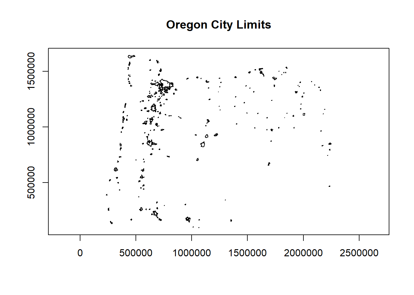

options(scipen=3)
plot(citylims$geometry, axes=T, main='Oregon City Limits') # plot it!

2.1.2 `st_read` versus `read_sf`

Above, I didn’t pass any parameters to st_read - typically I would pass the parameters quiet=TRUE and stringsAsFactors=FALSE - why would this be a good practice in general?

2.1.3 Answer

read_sf is an sf alternative to st_read (see this section 1.2.2). Try reading in citylims data above using read_sf and notice difference, and check out help(read_sf). read_sf and writesf` are simply aliases for st_read and st_write with modified default arguments. Big differences are:

stringsAsFactors=FALSE
quiet=TRUE
as_tibble=TRUE

2.1.4 Geodatabases

We use st_read or read_sf similarly for reading in an ESRI file geodatabase feature:

# download.file("ftp://ftp.gis.oregon.gov/adminbound/OregonStateParks_20181010.zip", "OregonStateParks.zip")
# unzip("OregonStateParks.zip", exdir = ".")
library(ggplot2)
fgdb = "OregonStateParks_20181010.gdb"

# List all feature classes in a file geodatabase
st_layers(fgdb)

## Driver: OpenFileGDB 
## Available layers:
##   layer_name geometry_type features fields
## 1   LO_PARKS Multi Polygon      431     15

# Read the feature class
parks <- st_read(dsn=fgdb,layer="LO_PARKS")

## Reading layer `LO_PARKS' from data source `C:\Users\mweber\GitProjects\AWRA_2020_R_Spatial\OregonStateParks_20181010.gdb' using driver `OpenFileGDB'
## Simple feature collection with 431 features and 15 fields
## geometry type:  GEOMETRY
## dimension:      XY
## bbox:           xmin: 222821.4 ymin: 88699.71 xmax: 2243413 ymax: 1655108
## projected CRS:  NAD83(2011) / Oregon GIC Lambert (ft)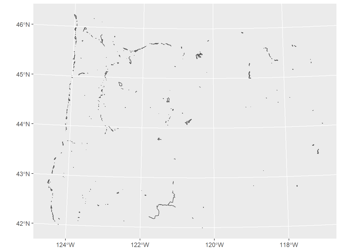

ggplot(parks) + geom_sf()

2.1.5 Geopackages

Another spatial file format is the geopackage. Let’s try a quick read and write of geopackage data. First we’ll read in a geopackage using data that comes with sf using dplyr syntax just to show something a bit different and use read_sf as an alternative to st_read. You may want to try writing the data back out as a geopackage as well.

Quick question: What are a couple advantages of geopackages over shapefiles?

library(dplyr)
nc <- system.file("gpkg/nc.gpkg", package="sf") %>% read_sf() # reads in
glimpse(nc)

## Rows: 100
## Columns: 15
## $ AREA      <dbl> 0.114, 0.061, 0.143, 0.070, 0.153, 0.097, 0.062, 0.091, 0...
## $ PERIMETER <dbl> 1.442, 1.231, 1.630, 2.968, 2.206, 1.670, 1.547, 1.284, 1...
## $ CNTY_     <dbl> 1825, 1827, 1828, 1831, 1832, 1833, 1834, 1835, 1836, 183...
## $ CNTY_ID   <dbl> 1825, 1827, 1828, 1831, 1832, 1833, 1834, 1835, 1836, 183...
## $ NAME      <chr> "Ashe", "Alleghany", "Surry", "Currituck", "Northampton",...
## $ FIPS      <chr> "37009", "37005", "37171", "37053", "37131", "37091", "37...
## $ FIPSNO    <dbl> 37009, 37005, 37171, 37053, 37131, 37091, 37029, 37073, 3...
## $ CRESS_ID  <int> 5, 3, 86, 27, 66, 46, 15, 37, 93, 85, 17, 79, 39, 73, 91,...
## $ BIR74     <dbl> 1091, 487, 3188, 508, 1421, 1452, 286, 420, 968, 1612, 10...
## $ SID74     <dbl> 1, 0, 5, 1, 9, 7, 0, 0, 4, 1, 2, 16, 4, 4, 4, 18, 3, 4, 1...
## $ NWBIR74   <dbl> 10, 10, 208, 123, 1066, 954, 115, 254, 748, 160, 550, 124...
## $ BIR79     <dbl> 1364, 542, 3616, 830, 1606, 1838, 350, 594, 1190, 2038, 1...
## $ SID79     <dbl> 0, 3, 6, 2, 3, 5, 2, 2, 2, 5, 2, 5, 4, 4, 6, 17, 4, 7, 1,...
## $ NWBIR79   <dbl> 19, 12, 260, 145, 1197, 1237, 139, 371, 844, 176, 597, 13...
## $ geom      <MULTIPOLYGON [°]> MULTIPOLYGON (((-81.47276 3..., MULTIPOLYGON...

2.1.6 Open spatial data sources

There is a wealth of open spatial data accessible online now via static URLs or APIs - a few examples include Data.gov, NASA SECAC Portal, Natural Earth, UNEP GEOdata, and countless others listed here at Free GIS Data

2.1.7 Spatial data from R packages

There are also a number of R packages written specifically to provide access to geospatial data - below are a few and we’ll step through some examples of pulling in data using some of these packages.

Table 2.1: Example R packages for spatial data retrieval.
Package name	Description
USABoundaries	Provide historic and contemporary boundaries of the US
tigris	Download and use US Census TIGER/Line Shapefiles in R
tidycensus	Uses Census American Community API to return tidyverse and optionally sf ready data frames
FedData	Functions for downloading geospatial data from several federal sources
elevatr	Access elevation data from various APIs (by Jeff Hollister)
getlandsat	Provides access to Landsat 8 data.
osmdata	Download and import of OpenStreetMap data.
raster	The `getData()` function downloads and imports administrative country, SRTM/ASTER elevation, WorldClim data.
rnaturalearth	Functions to download Natural Earth vector and raster data, including world country borders.
rnoaa	An R interface to National Oceanic and Atmospheric Administration (NOAA) climate data.
rWBclimate	An access to the World Bank climate data.

Below is an example of pulling in US states using the rnaturalearth package - note that the default is to pull in data as sp objects and we coerce to sf. Also take a look at the chained operation using dplyr. Try changing the filter or a parameter in ggplot.

library(rnaturalearth)
library(dplyr)
library(ggplot2)
states <- ne_states(country = 'United States of America')
states_sf <- st_as_sf(states)
states_sf %>%
  dplyr::filter(!name %in% c('Hawaii','Alaska') & !is.na(name)) %>%
  ggplot + geom_sf()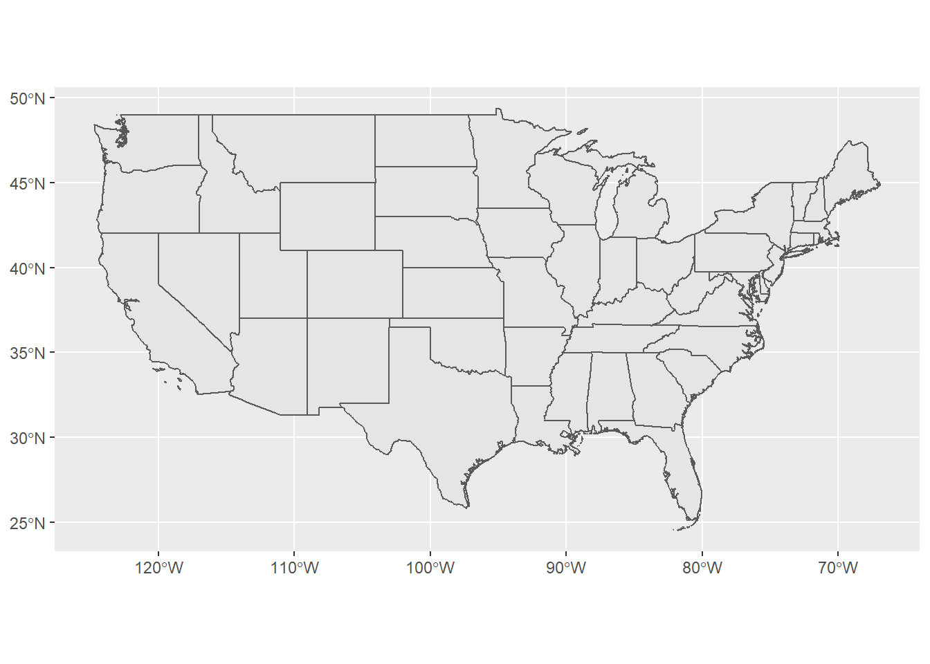

2.1.8 Read in raster data

Here we use the getData function in the raster package to download elevation into a RasterLayer and grab administrative boundaries from a database of global administrative boundaries - warning: sometimes getData function has trouble accessing the server and download can be a bit slow. Here we see as well how we can use vector spataio polygon data to crop raster data.

library(raster)
US <- getData("GADM",country="USA",level=2)
Benton <- US[US$NAME_1=='Oregon' & US$NAME_2=='Benton',]
elev <- getData('SRTM', lon=-123, lat=44)
elev <- crop(elev, Benton)
elev <- mask(elev, Benton)
plot(Benton, main="Elevation (m) in Benton County, Oregon", axes=T)
plot(elev, add=TRUE)
plot(Benton, add=TRUE)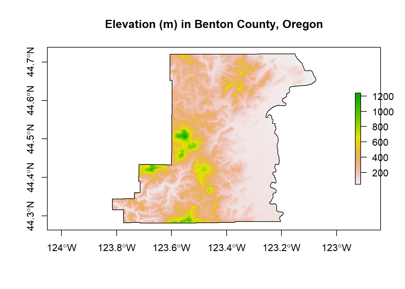

2.1.9 Read in OpenStreetMap data

The osmdata package is a fantastic resource for leveraging the OpenStreetMap (OSM) database.

library(osmdata)
library(mapview)

footway <- opq(bbox = "corvallis oregon") %>% 
  add_osm_feature(key = "highway", value = "footway") %>% 
  osmdata_sf()
footway <- footway$osm_lines
mapview(footway$geometry)

library(osmdata)
library(mapview)
rstrnts <- opq(bbox = "corvallis oregon") %>% 
    add_osm_feature(key = "amenity", value = "restaurant") %>%
    osmdata_sf()
rstrnts <- rstrnts$osm_points

mapview(rstrnts$geometry)

We often have flat files, locally on our machine or accessed elsewhere, that have coordinate information which we would like to make spatial:

library(devtools)
library(readr)
library(ggplot2)
# install_github("mhweber/awra2020spatial", force=TRUE)
library(awra2020spatial)
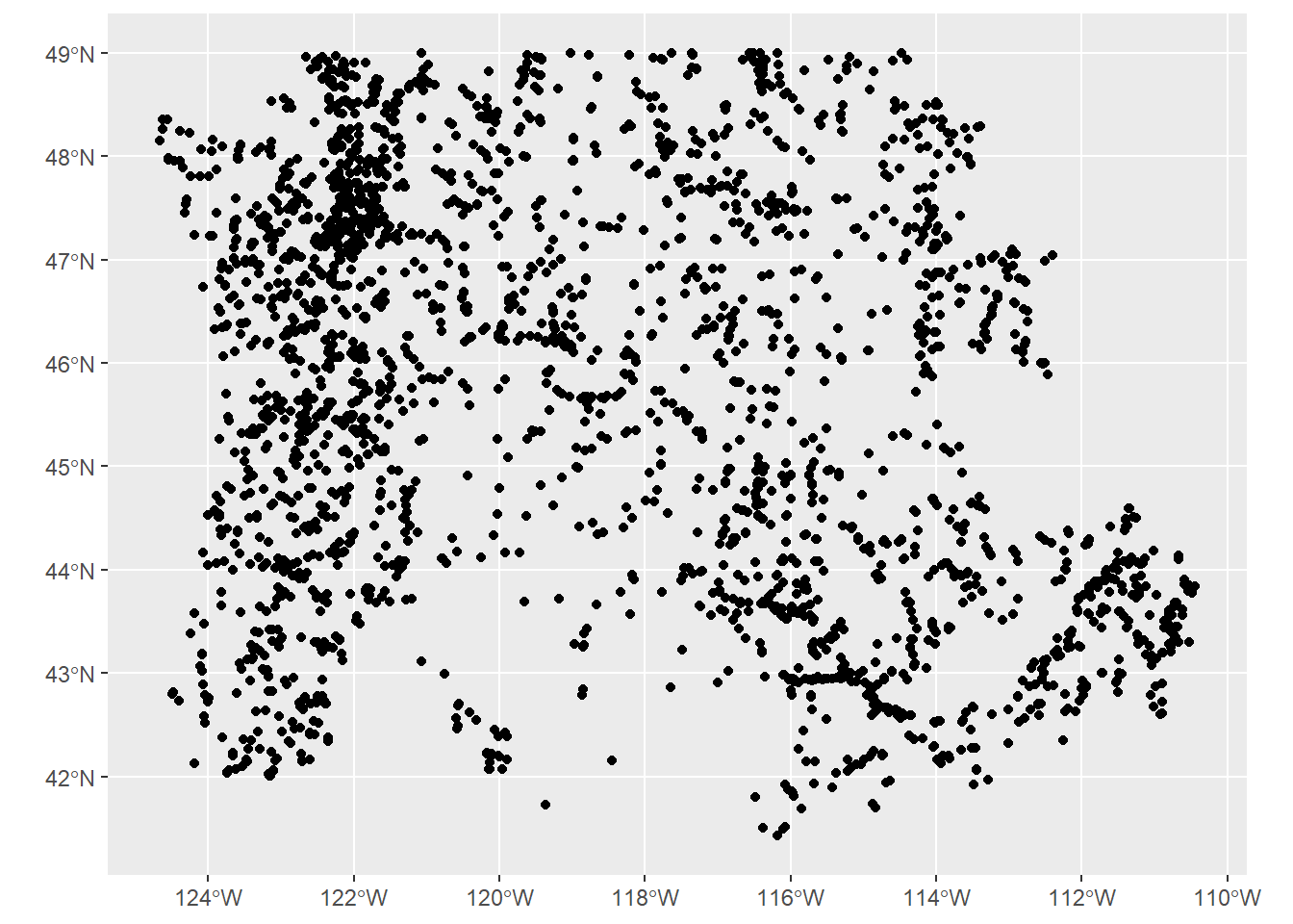
gages = read_csv(system.file("extdata/Gages_flowdata.csv", package = "awra2020spatial"))

gages_sf <- gages %>%
  st_as_sf(coords = c("LON_SITE", "LAT_SITE"), crs = 4269, remove = FALSE) %>%
  dplyr::select(STATION_NM,LON_SITE, LAT_SITE)

ggplot() + geom_sf(data=gages_sf)