Chapter 6 Geoprocessing

6.1 Lesson Goals

A quick look at a couple typical topological operations (spatial subsetting, spatial joins, dissolve) using sf

6.2 Example one

6.2.1 Spatial Subsetting

Let’s look at the bike paths and parks data in the awra2020spatial package. A typical spatial question we might ask of our data is ‘what trails go through parks in town?’ A great feature of sf is it supports spatial indexing:

library(sf)
library(awra2020spatial)
data(parks)
data(bike_paths)

plot(bike_paths$geoms, col='green', axes=T)
plot(parks$geoms, col='blue', add=T)
paths_in_parks <- bike_paths[parks,]
plot(paths_in_parks$geoms, col='red', lwd = 2, add=T)
title(main='Bike Paths in Parks in Austin')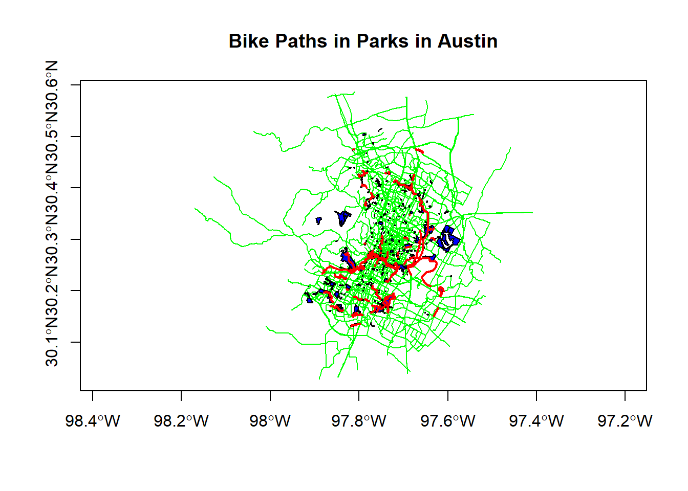

6.3 Example two

6.3.1 Spatial Join

First we’ll use chained operations to select just a couple columns from both bike_paths and parks, and then we’ll do a spatial join operation in sf. Note again, when we do a select on just attribute column, the geometry column remains - geometry is sticky in sf!

library(dplyr)
bike_paths <- bike_paths %>% 
  dplyr::select(ROUTE_NAME)
parks <- parks %>% 
  dplyr::select(LOCATION_NAME, ZIPCODE,PARK_TYPE)
parks_bike_paths <- st_join(parks, bike_paths) # st_intersects is the default
glimpse(parks_bike_paths)

## Rows: 606
## Columns: 5
## $ LOCATION_NAME <chr> "Stratford Overlook Greenbelt", "Highland Neighborhoo...
## $ ZIPCODE       <chr> "78746", "78752", "78703", "78753", "78724", "78702",...
## $ PARK_TYPE     <chr> "Greenbelt", "Neighborhood", "Pocket", "Neighborhood"...
## $ ROUTE_NAME    <chr> NA, NA, NA, NA, NA, NA, "TOWN LAKE HIKE & BIKE TRAIL"...
## $ geoms         <MULTIPOLYGON [°]> MULTIPOLYGON (((-97.78802 3..., MULTIPOL...

6.4 Example Three

6.4.1 Dissolve

We can perform a spatial dissolve in sf using dplyr group_by and summarize functions with an sf object! Note that we could pull down tidycensus at tract level, but instead we want to look at running a dissolve to get from block group to tract level

library(ggplot2)
parks$AREA <- st_area(parks)
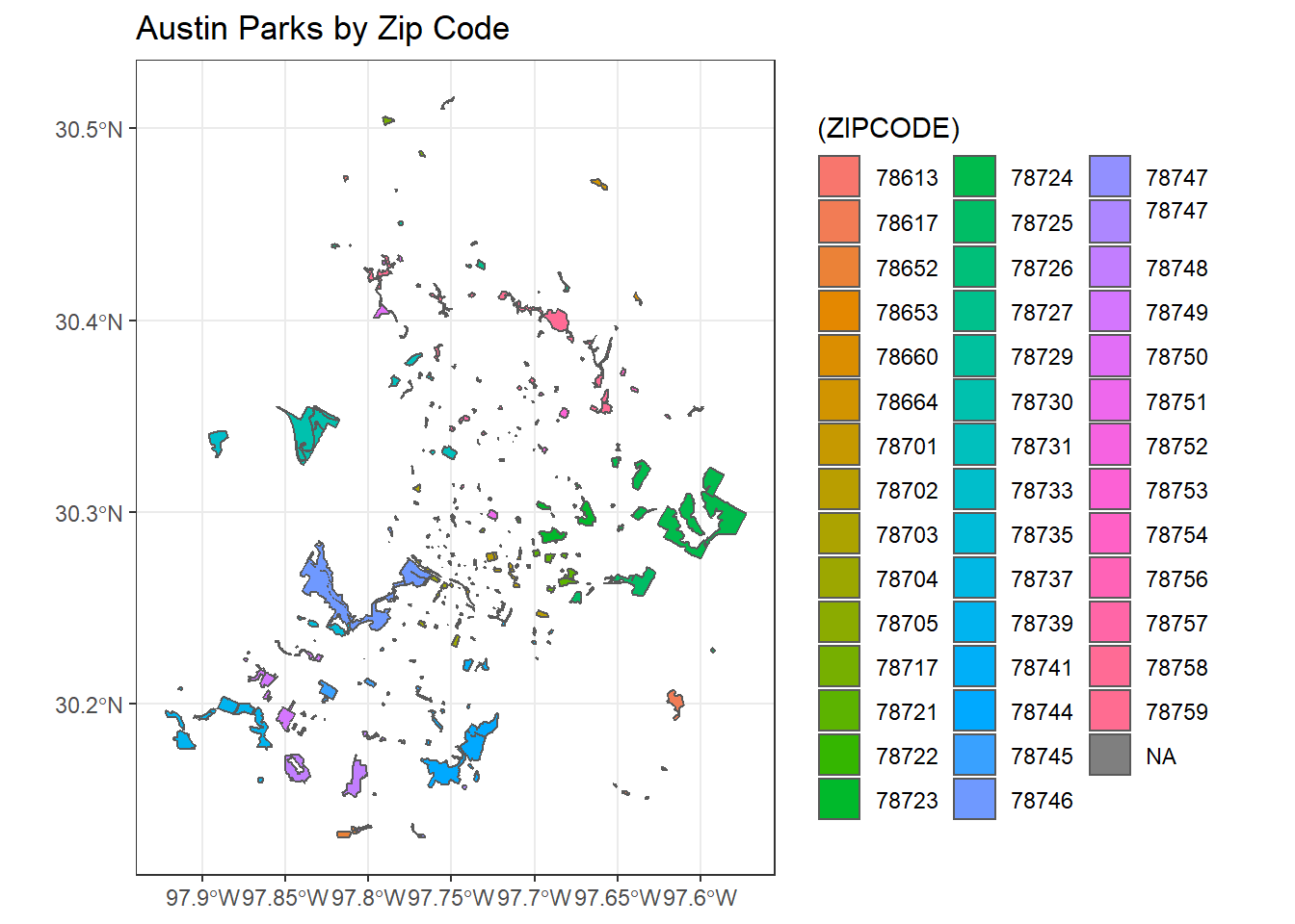
parks_zip <- parks %>% 
  group_by(ZIPCODE) %>%
  summarise(AREA = sum(AREA)) %>%
  ggplot() + geom_sf(aes(fill=(ZIPCODE))) +
  ggtitle("Austin Parks by Zip Code") + 
  theme_bw()
parks_zip