Chapter 2 Reading in Spatial Data
- There are several ways we typically get spatial data into R:
- Load spatial files we have on our machine or from remote source
- Load spatial data that is part of an R package
- Grab data using API (often making use of particular R packages)
- Converting flat files with x,y data to spatial data
- Geocoding data (we saw example of this at beginning)
For reading and writing vector and raster data in R, the several main packages we’ll look at are:
sforrgdalfor vector formats such as ESRI Shapefiles, GeoJSON, and GPX -sfuses OGR, which is a library under the GDAL source tree,under the hoodterra,raster, orstarsfor raster formats such as GeoTIFF or ESRI or ASCII grid using GDAL under the hood
We can quickly discover supported I/O vector formats either via sf or rgdal:
library(knitr)
library(sf)
library(rgdal)
print(paste0('There are ',st_drivers("vector") %>% nrow(), ' vector drivers available using st_read or read_sf'))
## [1] "There are 89 vector drivers available using st_read or read_sf"kable(head(ogrDrivers(),n=5))| name | long_name | write | copy | isVector |
|---|---|---|---|---|
| AeronavFAA | Aeronav FAA | FALSE | FALSE | TRUE |
| AmigoCloud | AmigoCloud | TRUE | FALSE | TRUE |
| ARCGEN | Arc/Info Generate | FALSE | FALSE | TRUE |
| AVCBin | Arc/Info Binary Coverage | FALSE | FALSE | TRUE |
| AVCE00 | Arc/Info E00 (ASCII) Coverage | FALSE | FALSE | TRUE |
kable(head(st_drivers(what='vector'),n=5))| name | long_name | write | copy | is_raster | is_vector | vsi | |
|---|---|---|---|---|---|---|---|
| ESRIC | ESRIC | Esri Compact Cache | FALSE | FALSE | TRUE | TRUE | TRUE |
| FITS | FITS | Flexible Image Transport System | TRUE | FALSE | TRUE | TRUE | FALSE |
| PCIDSK | PCIDSK | PCIDSK Database File | TRUE | FALSE | TRUE | TRUE | TRUE |
| netCDF | netCDF | Network Common Data Format | TRUE | TRUE | TRUE | TRUE | FALSE |
| PDS4 | PDS4 | NASA Planetary Data System 4 | TRUE | TRUE | TRUE | TRUE | TRUE |
As well as I/O raster formats via sf:
print(paste0('There are ',st_drivers(what='raster') %>% nrow(), ' raster drivers available'))## [1] "There are 149 raster drivers available"kable(head(st_drivers(what='raster'),n=5))| name | long_name | write | copy | is_raster | is_vector | vsi | |
|---|---|---|---|---|---|---|---|
| VRT | VRT | Virtual Raster | TRUE | TRUE | TRUE | FALSE | TRUE |
| DERIVED | DERIVED | Derived datasets using VRT pixel functions | FALSE | FALSE | TRUE | FALSE | FALSE |
| GTiff | GTiff | GeoTIFF | TRUE | TRUE | TRUE | FALSE | TRUE |
| COG | COG | Cloud optimized GeoTIFF generator | FALSE | TRUE | TRUE | FALSE | TRUE |
| NITF | NITF | National Imagery Transmission Format | TRUE | TRUE | TRUE | FALSE | TRUE |
2.1 Reading in vector data
sf can be used to read numerous file types:
- Shapefiles
- Geodatabases
- Geopackages
- Geojson
- Spatial database files
2.1.1 Shapefiles
Typically working with vector GIS data we work with ESRI shapefiles or geodatabases - here we have an example of how one would read in a shapefile using sf:
# download.file("ftp://ftp.gis.oregon.gov/adminbound/citylim_2017.zip","citylim_2017.zip")
# unzip("citylim_2017.zip", exdir = ".")
library(sf)
citylims <- st_read("citylim_2017.shp")
## Reading layer `citylim_2017' from data source
## `C:\Users\mweber\GitProjects\R-User-Group-Spatial-Workshop-2021\citylim_2017.shp'
## using driver `ESRI Shapefile'
## Simple feature collection with 241 features and 14 fields
## Geometry type: MULTIPOLYGON
## Dimension: XY
## Bounding box: xmin: 234278.9 ymin: 94690.89 xmax: 2249460 ymax: 1644089
## Projected CRS: NAD83 / Oregon GIC Lambert (ft)options(scipen=3)
plot(citylims$geometry, axes=T, main='Oregon City Limits') # plot it!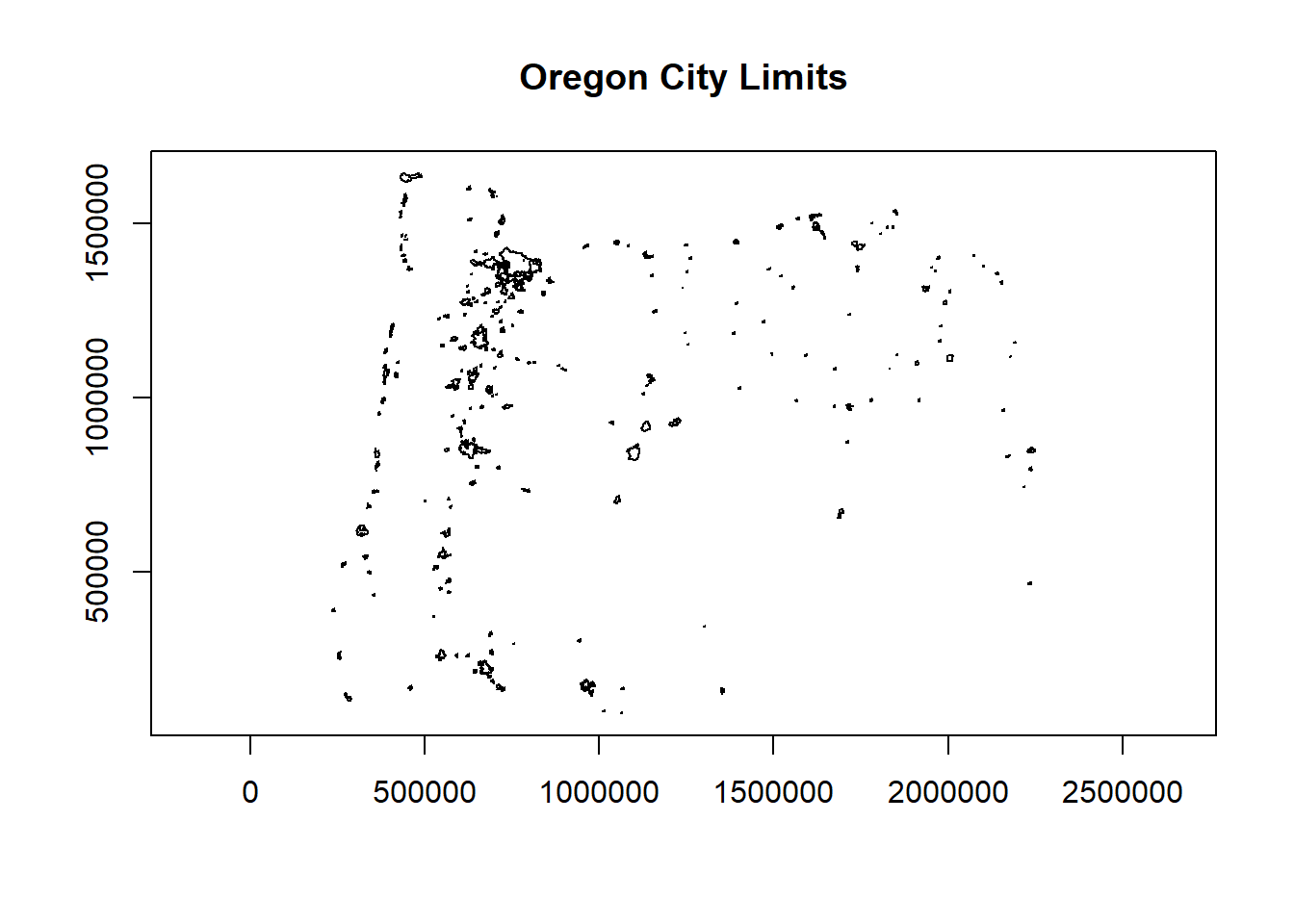
2.1.1.1 Exercise
st_read versus read_sf - above, I didn’t pass any parameters to st_read - typically I would pass the parameters quiet=TRUE and stringsAsFactors=FALSE - why would this be a good practice in general?
2.1.1.1.1 Solution
read_sf is an sf alternative to st_read (see this section 1.2.2). Try reading in citylims data above using read_sf and notice difference, and check out help(read_sf). read_sf and write_sf are simply aliases for st_read and st_write with modified default arguments. Big differences are:
- stringsAsFactors=FALSE
- quiet=TRUE
- as_tibble=TRUE
2.1.2 Geodatabases
We use st_read or read_sf similarly for reading in an ESRI file geodatabase feature:
# download.file("ftp://ftp.gis.oregon.gov/adminbound/OregonStateParks_20181010.zip", "OregonStateParks.zip")
# unzip("OregonStateParks.zip", exdir = ".")
library(ggplot2)
fgdb = "OregonStateParks_20181010.gdb"

# List all feature classes in a file geodatabase
st_layers(fgdb)
## Driver: OpenFileGDB
## Available layers:
## layer_name geometry_type features fields
## 1 LO_PARKS Multi Polygon 431 15# Read the feature class
parks <- st_read(dsn=fgdb,layer="LO_PARKS")## Reading layer `LO_PARKS' from data source
## `C:\Users\mweber\GitProjects\R-User-Group-Spatial-Workshop-2021\OregonStateParks_20181010.gdb'
## using driver `OpenFileGDB'
## Simple feature collection with 431 features and 15 fields
## Geometry type: GEOMETRY
## Dimension: XY
## Bounding box: xmin: 222821.4 ymin: 88699.71 xmax: 2243413 ymax: 1655108
## Projected CRS: NAD83(2011) / Oregon GIC Lambert (ft)ggplot(parks) + geom_sf()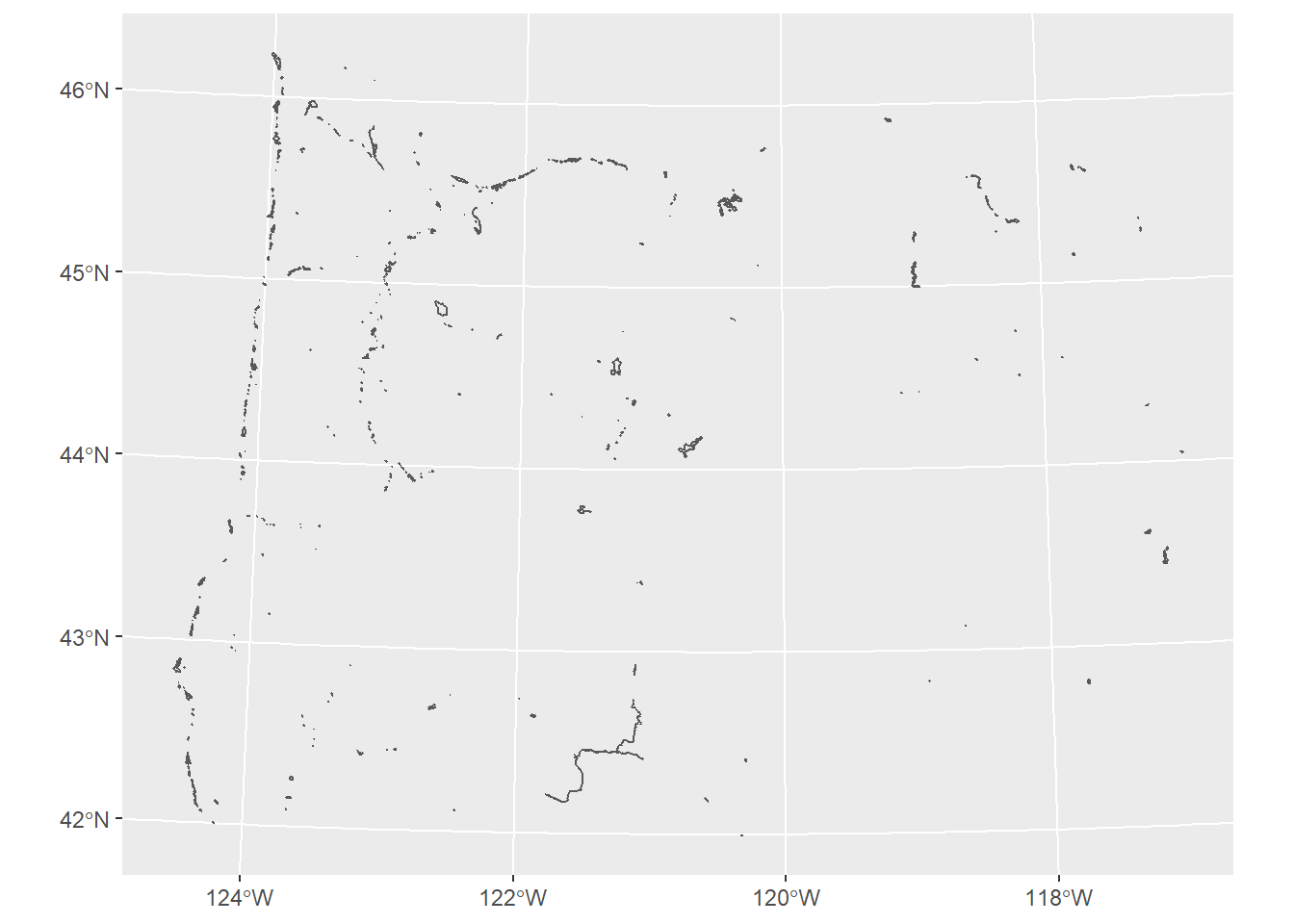
2.1.3 Geopackages
Another spatial file format is the geopackage. Let’s try a quick read and write of geopackage data. First we’ll read in a geopackage using data that comes with sf using dplyr syntax just to show something a bit different and use read_sf as an alternative to st_read. You may want to try writing the data back out as a geopackage as well.
library(dplyr)
nc <- system.file("gpkg/nc.gpkg", package="sf") %>% read_sf() # reads in
glimpse(nc)
## Rows: 100
## Columns: 15
## $ AREA <dbl> 0.114, 0.061, 0.143, 0.070, 0.153, 0.097, 0.062, 0.091, 0.11~
## $ PERIMETER <dbl> 1.442, 1.231, 1.630, 2.968, 2.206, 1.670, 1.547, 1.284, 1.42~
## $ CNTY_ <dbl> 1825, 1827, 1828, 1831, 1832, 1833, 1834, 1835, 1836, 1837, ~
## $ CNTY_ID <dbl> 1825, 1827, 1828, 1831, 1832, 1833, 1834, 1835, 1836, 1837, ~
## $ NAME <chr> "Ashe", "Alleghany", "Surry", "Currituck", "Northampton", "H~
## $ FIPS <chr> "37009", "37005", "37171", "37053", "37131", "37091", "37029~
## $ FIPSNO <dbl> 37009, 37005, 37171, 37053, 37131, 37091, 37029, 37073, 3718~
## $ CRESS_ID <int> 5, 3, 86, 27, 66, 46, 15, 37, 93, 85, 17, 79, 39, 73, 91, 42~
## $ BIR74 <dbl> 1091, 487, 3188, 508, 1421, 1452, 286, 420, 968, 1612, 1035,~
## $ SID74 <dbl> 1, 0, 5, 1, 9, 7, 0, 0, 4, 1, 2, 16, 4, 4, 4, 18, 3, 4, 1, 1~
## $ NWBIR74 <dbl> 10, 10, 208, 123, 1066, 954, 115, 254, 748, 160, 550, 1243, ~
## $ BIR79 <dbl> 1364, 542, 3616, 830, 1606, 1838, 350, 594, 1190, 2038, 1253~
## $ SID79 <dbl> 0, 3, 6, 2, 3, 5, 2, 2, 2, 5, 2, 5, 4, 4, 6, 17, 4, 7, 1, 0,~
## $ NWBIR79 <dbl> 19, 12, 260, 145, 1197, 1237, 139, 371, 844, 176, 597, 1369,~
## $ geom <MULTIPOLYGON [°]> MULTIPOLYGON (((-81.47276 3..., MULTIPOLYGON ((~2.1.3.1 Exercise
What are a couple advantages of geopackages over shapefiles?
2.1.3.2 Solution
Some thoughts here, main ones probably:
- geopackages avoid mult-file format of shapefiles
- geopackages avoid the 2gb limit of shapefiles
- geopackages are open-source and follow OGC standards
- lighter in file size than shapefiles
- geopackages avoid the 10-character limit to column headers in shapefile attribute tables (stored in archaic .dbf files)
2.1.4 Open spatial data sources
There is a wealth of open spatial data accessible online now via static URLs or APIs - a few examples include Data.gov, NASA SECAC Portal, Natural Earth, UNEP GEOdata, and countless others listed here at Free GIS Data
2.1.5 Spatial data from R packages
There are also a number of R packages written specifically to provide access to geospatial data - below are a few and we’ll step through some examples of pulling in data using some of these packages.
| Package name | Description |
|---|---|
| USABoundaries | Provide historic and contemporary boundaries of the US |
| tigris | Download and use US Census TIGER/Line Shapefiles in R |
| tidycensus | Uses Census American Community API to return tidyverse and optionally sf ready data frames |
| FedData | Functions for downloading geospatial data from several federal sources |
| elevatr | Access elevation data from various APIs (by Jeff Hollister) |
| getlandsat | Provides access to Landsat 8 data. |
| osmdata | Download and import of OpenStreetMap data. |
| raster | The getData() function downloads and imports administrative country, SRTM/ASTER elevation, WorldClim data. |
| rnaturalearth | Functions to download Natural Earth vector and raster data, including world country borders. |
| rnoaa | An R interface to National Oceanic and Atmospheric Administration (NOAA) climate data. |
| rWBclimate | An access to the World Bank climate data. |
Below is an example of pulling in US states using the rnaturalearth package - note that the default is to pull in data as sp objects and we coerce to sf. Also take a look at the chained operation using dplyr. Try changing the filter or a parameter in ggplot.
library(rnaturalearth)
library(dplyr)
states <- ne_states(country = 'United States of America')
states_sf <- st_as_sf(states)
states_sf %>%
  dplyr::filter(!name %in% c('Hawaii','Alaska') & !is.na(name)) %>%
  ggplot + geom_sf()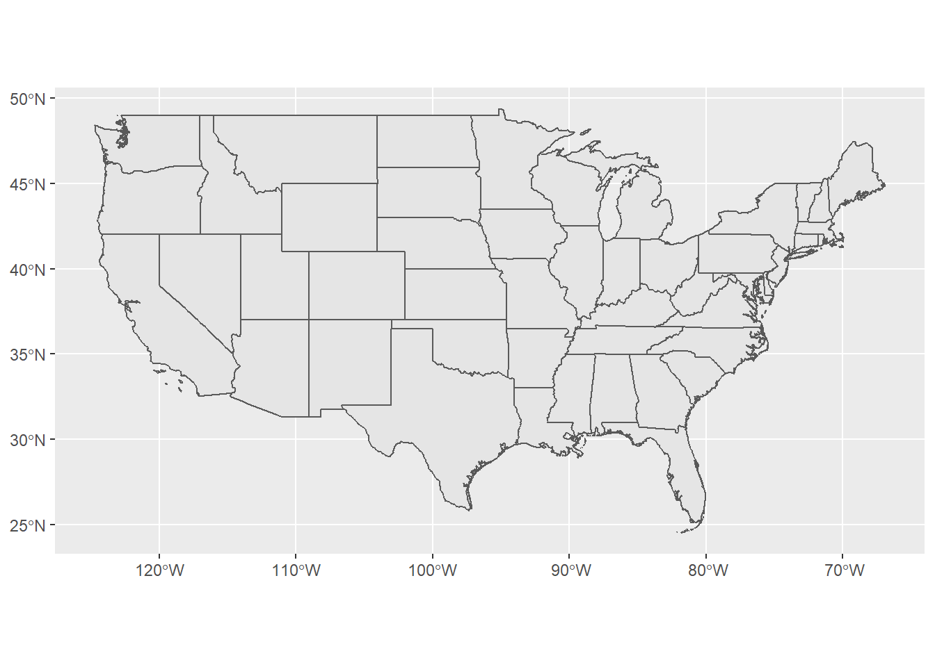
2.1.6 Read in OpenStreetMap data
The osmdata package is a fantastic resource for leveraging the OpenStreetMap (OSM) database.
First we’ll find available tags to get foot paths to plot
library(osmdata)
library(mapview)

head(available_tags("highway")) # get rid of head when you run - just used to truncate output
## [1] "bridleway" "bus_guideway" "bus_stop" "busway" "construction"
## [6] "corridor"footway <- opq(bbox = "corvallis oregon") %>%
add_osm_feature(key = "highway", value = c("footway","cycleway","path", "path","pedestrian","track")) %>%
osmdata_sf()
footway <- footway$osm_lines
rstrnts <- opq(bbox = "corvallis oregon") %>%
add_osm_feature(key = "amenity", value = "restaurant") %>%
osmdata_sf()
rstrnts <- rstrnts$osm_points
mapview(footway$geometry) + mapview(rstrnts)Take a minute and try pulling in data of your own for your own area and plotting using osmdata
2.2 Raster data
2.2.1 raster package
Here we use the getData function in the raster package to download elevation into a RasterLayer and grab administrative boundaries from a database of global administrative boundaries - warning: sometimes getData function has trouble accessing the server and download can be a bit slow. Here we see as well how we can use vector spataio polygon data to crop raster data.
library(raster)
US <- getData("GADM",country="USA",level=2)
Benton <- US[US$NAME_1=='Oregon' & US$NAME_2=='Benton',]
elev <- getData('SRTM', lon=-123, lat=44)
elev <- crop(elev, Benton)
elev <- mask(elev, Benton)
plot(Benton, main="Elevation (m) in Benton County, Oregon", axes=T)
plot(elev, add=TRUE)
plot(Benton, add=TRUE)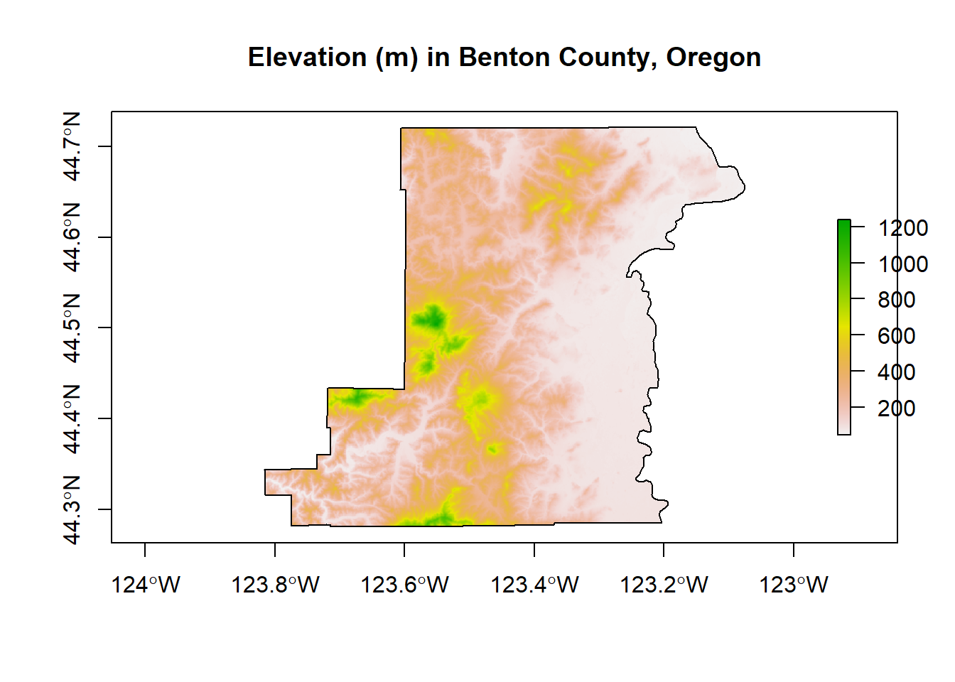
2.2.2 terra package
Load stock elevation .tif file that comes with package
library(terra)
f <- system.file("ex/elev.tif", package="terra")
elev <- rast(f)
barplot(elev, digits=-1, las=2, ylab="Frequency")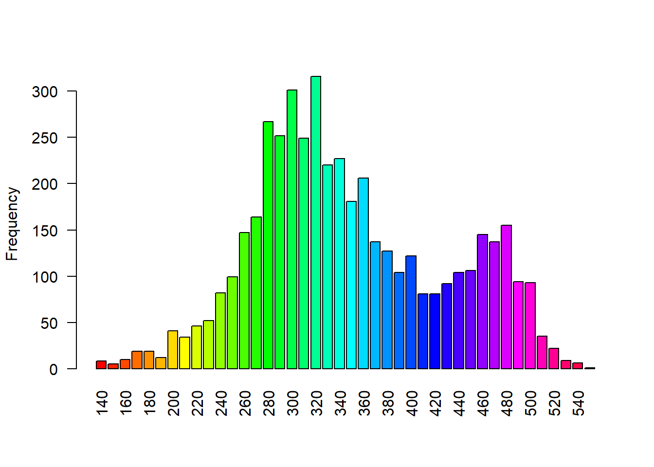
plot(elev)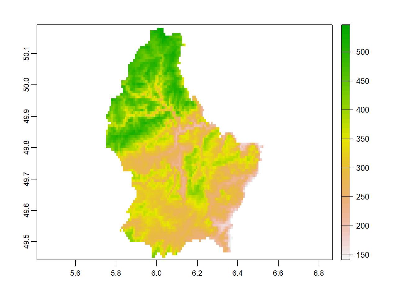
2.2.3 stars package
Load stock Landsat 7 .tif file that comes with package
library(stars)
tif = system.file("tif/L7_ETMs.tif", package = "stars")
read_stars(tif) %>%
  dplyr::slice(index = 1, along = "band") %>%
  plot()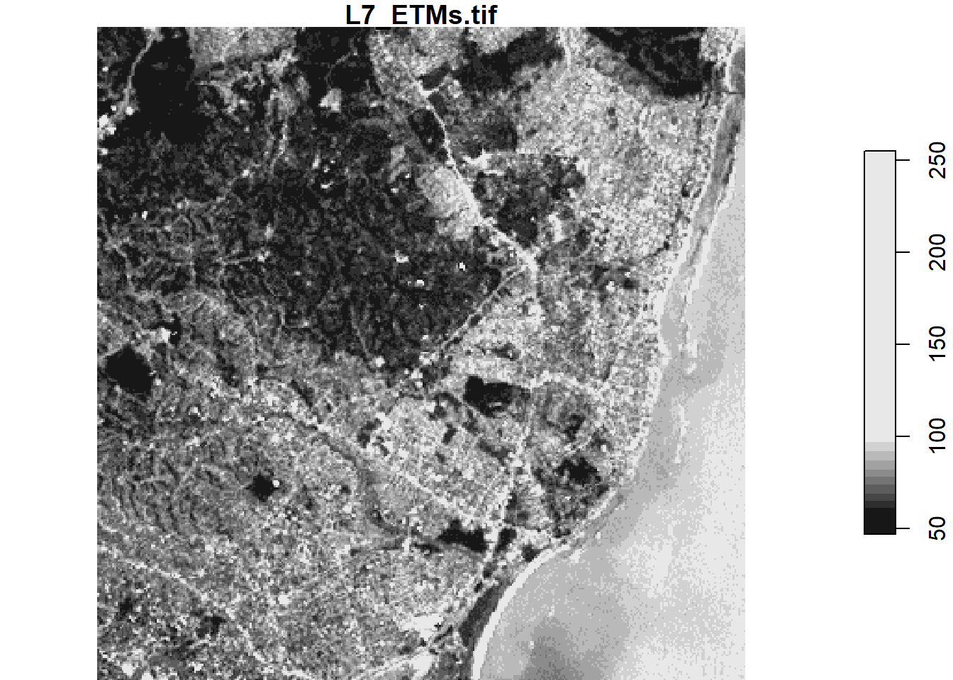
We’ll get a sense for what ‘slice’ and ‘index’ above are doing in the Raster data section
2.3 Convert flat files to spatial
We often have flat files, locally on our machine or accessed elsewhere, that have coordinate information which we would like to make spatial.
In the steps below, we
- read in a .csv file of USGS gages in the PNW that have coordinate columns
- Use
st_as_sffunction insfto convert the data frame to ansfspatial simple feature collection by:- passing the coordinate columns to the coords parameter
- specifying a coordinate reference system (CRS)
- opting to retain the coordinate columns as attribute columns in the resulting
sffeature collection.
- Keep only the coordinates and station ID in resulting
sffeature collection, and - Plotting our gages as spatial features with
ggplot2usinggeom_sf.
library(readr)
library(ggplot2)
library(Rspatialworkshop)
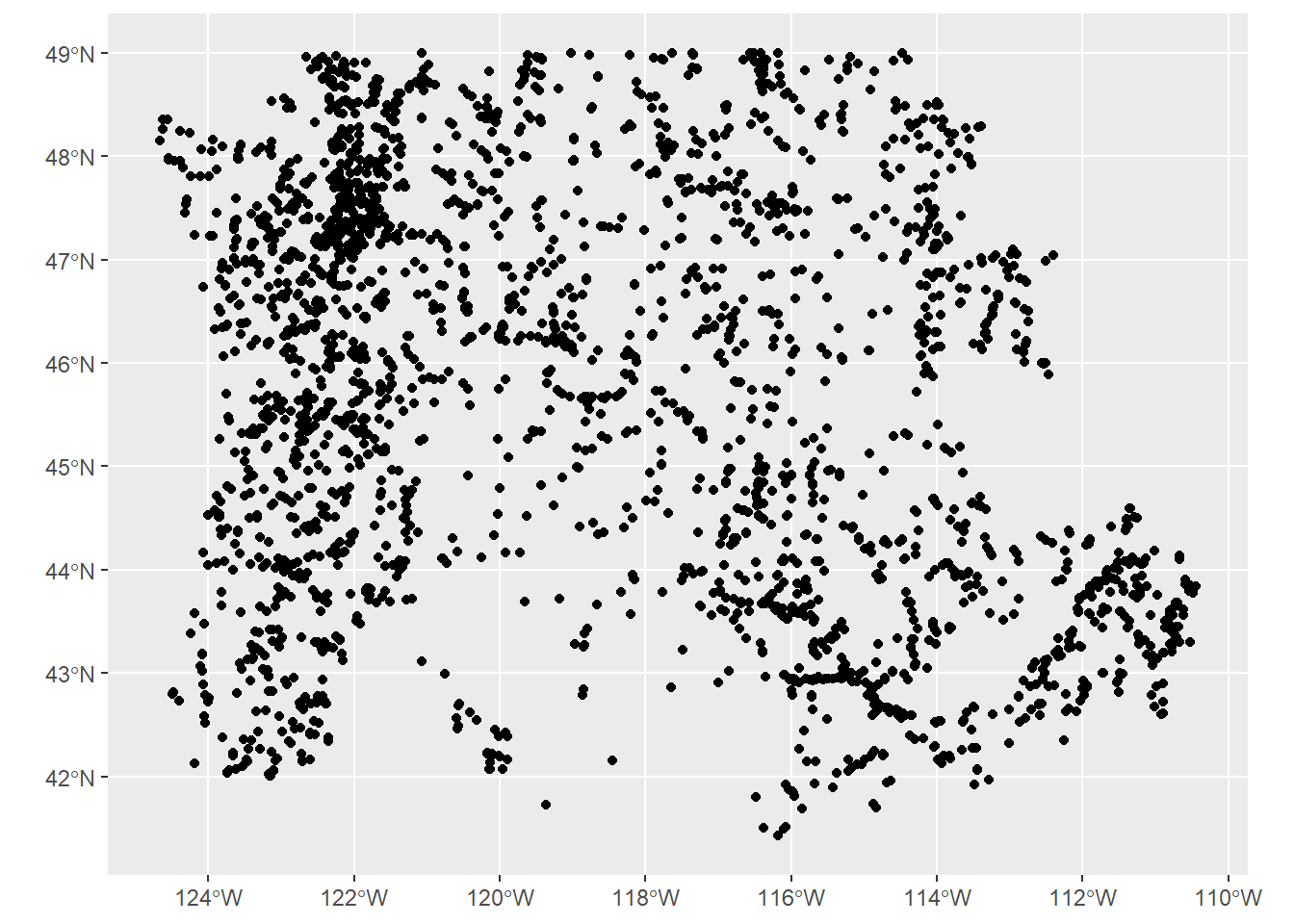
gages = read_csv(system.file("extdata/Gages_flowdata.csv", package = "Rspatialworkshop"))
gages_sf <- gages %>%
st_as_sf(coords = c("LON_SITE", "LAT_SITE"), crs = 4269, remove = FALSE) %>%
dplyr::select(STATION_NM,LON_SITE, LAT_SITE)
ggplot() + geom_sf(data=gages_sf)