Chapter 6 Geoprocessing
6.1 Lesson Goals
A quick look at a some typical topological operations (spatial subsetting, spatial joins, dissolve) using sf - followed by a couple ‘real world’ spatial tasks. We’ll be using several of the geometric binary predicates described in ?sf::geos_binary_pred.
6.2 Spatial Subsetting
Let’s look at the bike paths and parks data in the Rspatialworkshop package. There are sf feature collections of parks and trails in Austin in the package - we want to know what bike trails go through parks. A great feature of sf is it supports spatial indexing:
library(sf)
library(Rspatialworkshop)
data(parks)
data(bike_paths)

plot(bike_paths$geoms, col='green', axes=T)
plot(parks$geoms, col='blue', add=T)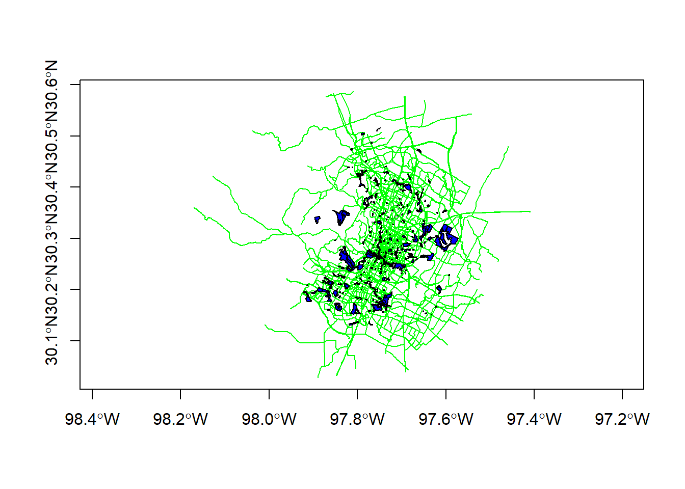
paths_in_parks <- bike_paths[parks,]plot(parks$geoms, col='blue', axes=T)
plot(paths_in_parks$geoms, col='red', lwd = 2, add=T)
title(main='Bike Paths in Parks in Austin')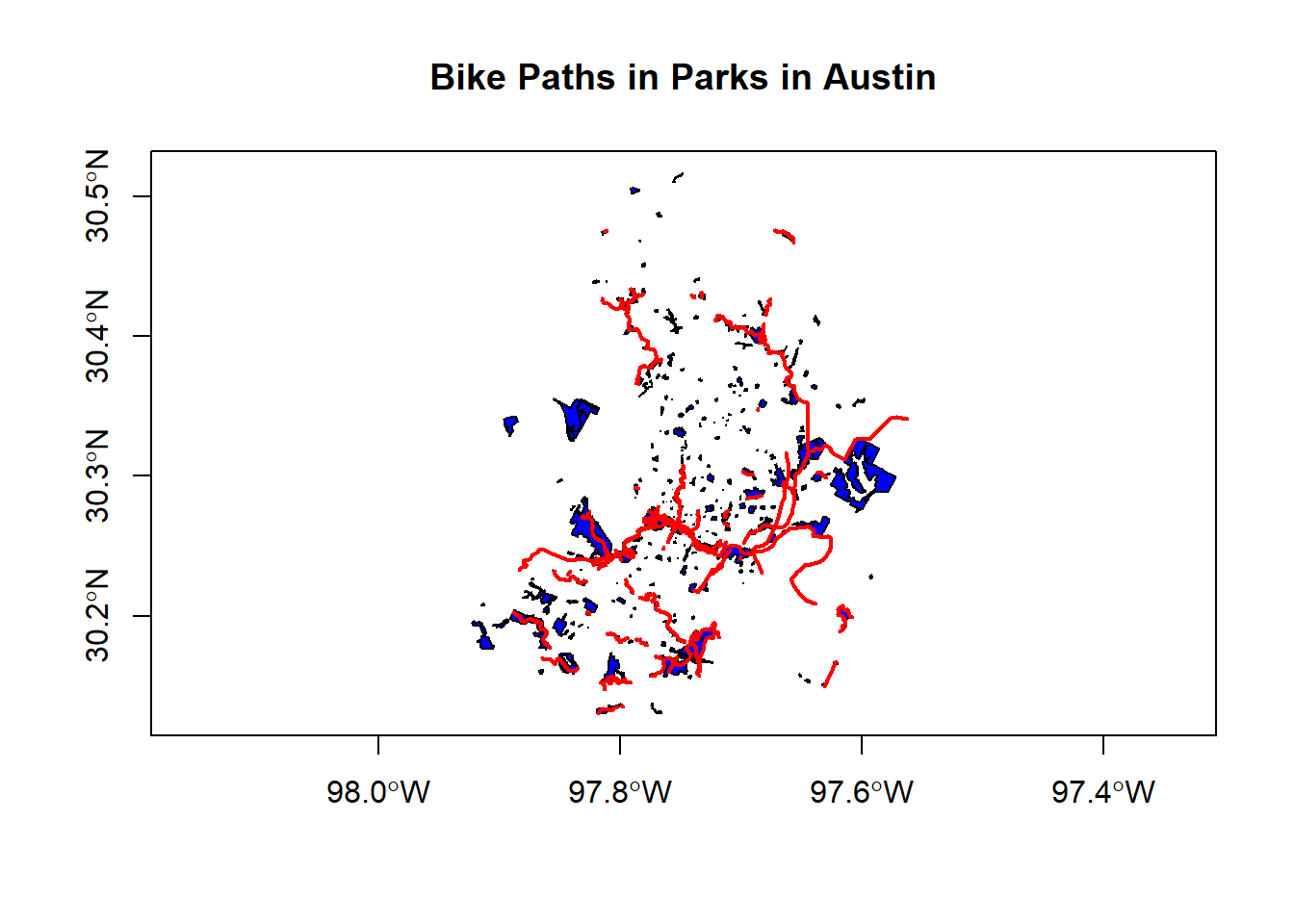
6.3 Spatial Join
We’ll use chained operations to select just a couple columns from both bike_paths and parks, and then we’ll do a spatial join operation with sf. Note that when we do a select on just attribute column, the geometry column remains - geometry is sticky in sf!
library(dplyr)
bike_paths <- bike_paths %>%
  dplyr::select(ROUTE_NAME)
parks <- parks %>%
  dplyr::select(LOCATION_NAME, ZIPCODE,PARK_TYPE)
parks_bike_paths <- st_join(parks, bike_paths) # st_intersects is the default
glimpse(parks_bike_paths)
## Rows: 744
## Columns: 5
## $ LOCATION_NAME <chr> "Stratford Overlook Greenbelt", "Highland Neighborhood P~
## $ ZIPCODE <chr> "78746", "78752", "78703", "78753", "78724", "78702", "7~
## $ PARK_TYPE <chr> "Greenbelt", "Neighborhood", "Pocket", "Neighborhood", "~
## $ ROUTE_NAME <chr> NA, NA, NA, NA, NA, NA, "TOWN LAKE HIKE & BIKE TRAIL", "~
## $ geoms <MULTIPOLYGON [°]> MULTIPOLYGON (((-97.78802 3..., MULTIPOLYGO~6.4 Dissolve
We can perform a spatial dissolve in sf using dplyr group_by and summarize functions with an sf object.
What we are doing here is using zip code as our grouping variable with dplyr, summarizing area using the sf st_area function at that grouping level, and mapping the result.
library(ggplot2)
parks$AREA <- st_area(parks)
parks_zip <- parks %>%
  group_by(ZIPCODE) %>%
  summarise(AREA = sum(AREA)) %>%
  ggplot() + geom_sf(aes(fill=(ZIPCODE))) +
  ggtitle("Austin Parks by Zip Code") +
  theme_bw()
parks_zip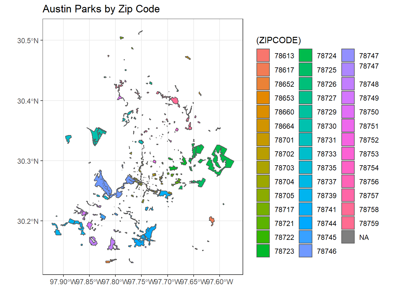
6.5 Spatial Overlap
Here’s a fun example using material posted by Nicholas Tierney here that he put together based on this Stack Overflow discussion.
First we’ll extract the Portland Oregon metropolitan area using the tidycensus and tigris packages
library(ggplot2)
library(tidycensus)
library(tidyverse)
library(tigris)

tracts <- get_acs(geography = "tract", variables = "DP04_0134",
                state = "OR", geometry = TRUE, progress_bar = FALSE)

pdx <- core_based_statistical_areas(cb = TRUE, progress_bar = FALSE) %>%
  filter(GEOID == "38900")
ggplot() +
  geom_sf(data = pdx,
fill = "forestgreen") 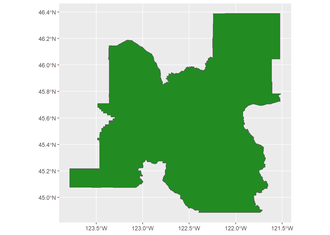
6.5.1 Next we’ll create a dummy spatial polygon file to compare area with using the rmapshaper package to simplify the border of the PDX metropolitan polygon
library(rmapshaper)
pdx_simplified <- pdx %>%
  ms_simplify(keep = 0.01)
6.5.2 Then we can overlay polygons in ggplot to see how similar they are, showing the original census PDX metropolitan area in green, and new simplified polygon in red
ggplot() +
  geom_sf(data = pdx,
          fill = "forestgreen", alpha = 0.5) +
  geom_sf(data = pdx_simplified,
          fill = "firebrick",
          alpha = 0.5)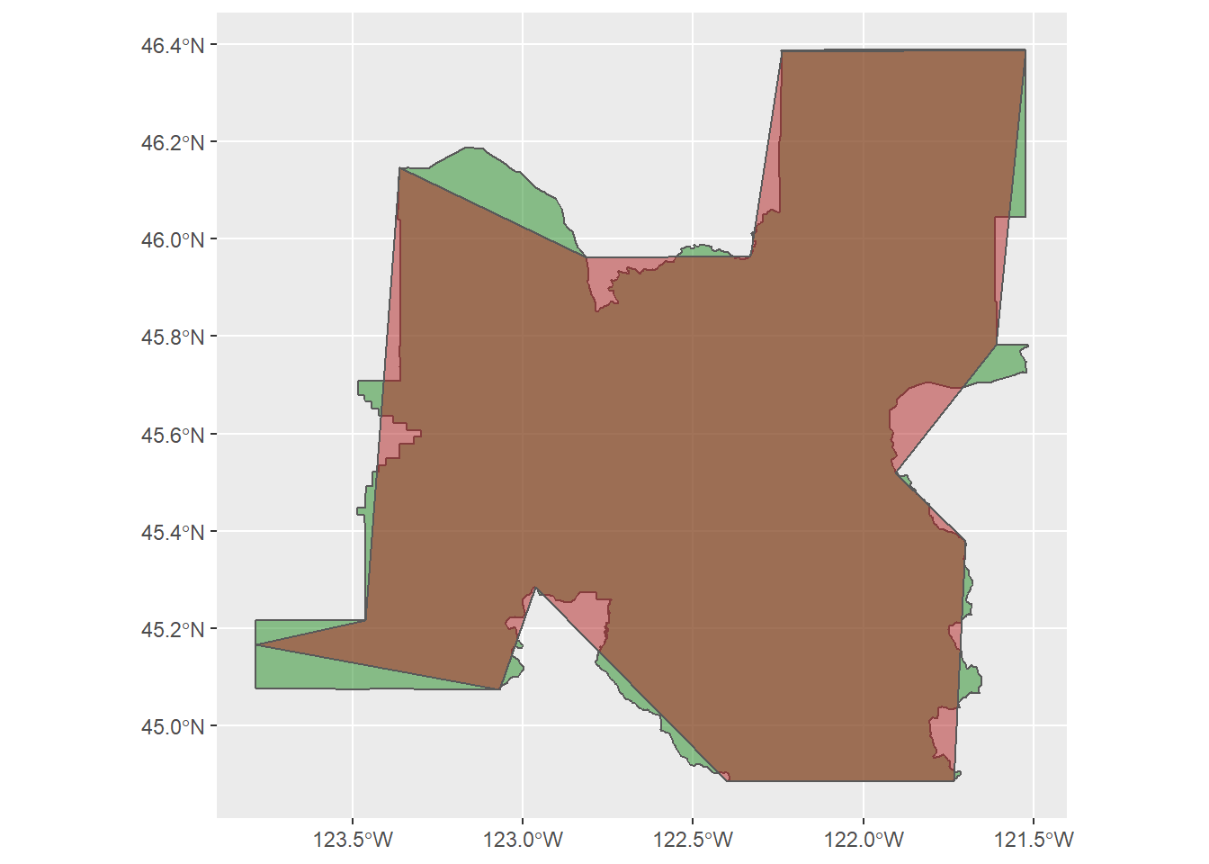
6.5.3 Now that we have an original and simplified polygon to compare, the process we want to use is:
- Calculate original metro area polygon area
- Calculate the intersection of these two areas - original and simplified (st_intersection)
- Calculate that area (st_area)
- Then only keep the relevant data again
We’ll run the steps then combine into a function
original_area <- pdx %>%
    mutate(original_area = st_area(.)) %>%
    dplyr::select(NAME, original_area) %>%
    st_drop_geometry()

intersection_area <- st_intersection(pdx, pdx_simplified) %>%
    mutate(intersect_area = st_area(.)) %>%
    dplyr::select(NAME, intersect_area) %>%
    st_drop_geometry()
6.5.4 Exercise
This step should have given you an error -THIS IS VERY COMMON WORKING WITH SPATIAL DATA IN R AND USING sf.
6.5.5 Solution
pdx_simplified <- st_make_valid(pdx_simplified)
pdx <- st_make_valid(pdx)

original_area <- pdx %>%
    mutate(original_area = st_area(.)) %>%
    dplyr::select(NAME, original_area) %>%
    st_drop_geometry()

intersection_area <- st_intersection(pdx, pdx_simplified) %>%
    mutate(intersect_area = st_area(.)) %>%
    dplyr::select(NAME, intersect_area) %>%
    st_drop_geometry()

# show the area of intersection
intersection_area
## NAME intersect_area
## 1 Portland-Vancouver-Hillsboro, OR-WA 16524152114 [m^2]# show the proportion of overlap
intersection_area %>%
left_join(original_area,
by = "NAME") %>%
mutate(orig = as.numeric(original_area),
new = as.numeric(intersect_area),
proportion = (new / orig) * 100)## NAME intersect_area original_area
## 1 Portland-Vancouver-Hillsboro, OR-WA 16524152114 [m^2] 17633108214 [m^2]
## orig new proportion
## 1 17633108214 16524152114 93.710946.5.6 Exercise
Why did I use as.numeric in the mutate statement above?
6.5.6.1 Solution
sf will calculate area or length for features as units - which is convenient and forces you to be up front about units used, but you when you do calculations with attributes stored as units the units are retained - which is often not what is desired. You can see this behavior using str(st_area(pdx)).
All steps rolled into a function
calculate_spatial_overlap <-
  function(shape_new,shape_old,     shared_column_name) {
    intersection_area <- st_intersection(shape_new, shape_old) %>%
    mutate(intersect_area = st_area(.)) %>%
    dplyr::select(shared_column_name, intersect_area) %>%
    st_drop_geometry()

  # Create a fresh area variable
  shape_old_areas <- shape_old %>%
    mutate(original_area = st_area(.)) %>%
    dplyr::select(original_area, shared_column_name) %>%
    st_drop_geometry()

  intersection_area %>%
    left_join(shape_old_areas,
              by = shared_column_name) %>%
    mutate(orig = as.numeric(original_area),
           new = as.numeric(intersect_area),
           proportion = (new / orig) * 100)

}

calculate_spatial_overlap(pdx, pdx_simplified, shared_column_name='NAME')
## NAME intersect_area original_area
## 1 Portland-Vancouver-Hillsboro, OR-WA 16524152114 [m^2] 17295383068 [m^2]
## orig new proportion
## 1 17295383068 16524152114 95.540836.6 Deriving data for a sites or a watershed
6.6.1 Extract using sites
First we’ll use dataRetrieval to find NWIS sites in Benton County Oregon
library(mapview)
library(dataRetrieval)
library(sf)
Benton_Stations <- readNWISdata(stateCd="Oregon", countyCd="Benton")
siteInfo <- attr(Benton_Stations , "siteInfo")
stations_sf = st_as_sf(siteInfo, coords = c("dec_lon_va", "dec_lat_va"), crs = 4269,agr = "constant")
mapview(stations_sf)
6.6.1.1 Exercise
What is the agr argument to st_as_sf in code chunk above?
6.6.1.2 Solution
Try help(st_sf) and look at details, and try demo(nc) to see a worked example. Basically, agr specifies the attribute-geometry relationship - does the attribute represent a constant value, an aggregation over the geometry, or an identity that uniquely identifies the geometry. For the most part I haven’t paid too much attention to this parameter but similar to units, it can help with constructing a more self-descriptive spatial object.
6.6.2 River reaches and basin
Next we’ll use nhdplusTools to get the river reaches for the Mary’s River in Benton county, get the watershed Mary’s River watershed, and then spatially subset the stations to the watershed
library(nhdplusTools)
start_comid = 23762881
nldi_feature <- list(featureSource = "comid", featureID = start_comid)

flowline_nldi <- navigate_nldi(nldi_feature, mode = "UT", data_source = "flowlines", distance=5000)

basin <- get_nldi_basin(nldi_feature = nldi_feature)
6.6.3 StreamCat data for watershed
StreamCat provides pre-compiled watershed metrics for every NHDPlus stream reach in the CONUS. Note that the StreamCatTools R package is in alpha development and will only work behind the EPA firewall at the moment (must be connected to VPN to use)
# install_github('USEPA/StreamCatTools')
library(StreamCatTools)
# get NHDPlus COMIDS for flowlines of the Mary's River - some machinations on our data from NLDI using nhdplusTools...
comids <- c(flowline_nldi$origin$comid,flowline_nldi$UT_flowlines$nhdplus_comid)
comids <- paste(comids,collapse=",",sep="")

df <- sc_get_data(metric='PctImp2011', aoi='catchment', comid=comids)
## &name=PctImp2011&comid=23762881,23762881,23764703,23762883,23765593,23764671,23762885,23764723,23764669,23764667,23762887,23764733,23764721,23764715,23764657,23764641,23764643,23764779,23762889,23764581,23764639,23764645,23762891,23764771,23762893,23764785,23762895,23762959,23764823,23764825,23762897,23764765,23764805,23762961,23764841,23762899,23762939,23764755,23764757,23764893,23762963,23762901,23763967,23762941,23764731,23764717,23764719,23764869,23762965,23762903,23764651,23763969,23764681,23762943,23764767,23764711,23764713,23764705,23764707,23764819,23762967,23764633,23762905,23763971,23764693,23762945,23764773,23764709,23764807,23763809,23762969,23762907,23764631,23763973,23762947,23764789,23764817,23764803,23764923,23762971,23762909,23764629,23764593,23764595,23763931,23762949,23764799,23764801,23763767,23762973,23762911,23764619,23764561,23764567,23764835,23763933,23762951,23764813,23764905,23763769,23762975,23764981,23762913,23764625,23763935,23764793,23764827,23762953,23764913,23763771,23762977,23762915,23764621,23763937,23764741,23764863,23762955,23764933,23764937,23763773,23764899,23762979,23762917,23764663,23764747,23763939,23764865,23764881,23762957,23763775,23764903,23762981,23762919,23762925,23764739,23764753,23763941,23764873,23764875,23763777,23764925,23762983,23762921,23764617,23763897,23762927,23765581,23763943,23762985,23762923,23764551,23764589,23764587,23764637,23762929,23764833,23764769,23762987,23764445,23764447,23764553,23764555,23762931,23763759,23762989,23762993,23764437,23764439,23764369,23764367,23764505,23764507,23764599,23762933,23763761,23765007,23762991,23765063,23762995,23764401,23764399,23764341,23762935,23764579,23763763,23764993,23765021,23765077,23765115,23765039,23762997,23764319,23764279,23762937,23764611,23763765,23764977,23764997,23765079,23765125,23765101,23762999,23765661,23764971,23764973,23765095,23765123,23765027,23763001,23764653,23763003,23764685,23763005,23764691,23764729,23764743,23764763&areaOfInterest=catchmentflowline_nldi$UT_flowlines$PCTIMP2011CAT <- df$PCTIMP2011CAT[match(flowline_nldi$UT_flowlines$nhdplus_comid, df$COMID)]
mapview(flowline_nldi$UT_flowlines, zcol = "PCTIMP2011CAT", legend = TRUE) + mapview(basin, alpha.regions=.07)6.7 Extract
Last, just quick examples of extracting raster values at points or using extract to summarize raster values for spatial polygons.
Extract of elevation for station points
library(FedData)
library(terra)
# The data access for elevation using FedData slow, so I've commented out and saved the data locally...

# elev <- get_ned(template = as(basin,'Spatial'),label='Marys River')
# marys_elev <- terra::crop(elev, basin)
# terra::writeRaster(marys_elev, 'C:/Users/mweber/Temp/marys_elev.tif')
marys_elev <- terra::rast('C:/Users/mweber/Temp/marys_elev.tif')

st_crs(stations_sf)$wkt == crs(marys_elev)
## [1] FALSEmarys_elev <- terra::project(marys_elev, st_crs(stations_sf)$wkt)
stations_sf$elevation <- terra::extract(marys_elev, vect(stations_sf))
stations_sf$elevation## ID marys_elev
## 1 1 88.02767
## 2 2 87.99461
## 3 3 74.26478
## 4 4 111.86833
## 5 5 70.22331
## 6 6 81.99174
## 7 7 59.63894
## 8 8 NaN
## 9 9 191.47162Elevation summary for the watershed - doing zonal statistics using a vector feature zone on a raster
# project both our raster and polygon data
library(terra)
basin <- st_transform(basin, 5070)
marys_elev <- project(marys_elev, st_crs(basin)$wkt, method = "bilinear")

meanelev <- terra::extract(marys_elev, vect(basin), fun = mean, na.rm = T, small = T)
meanelev
## ID marys_elev
## 1 1 227.784Categorical raster (NLCD) summary for the watershed
raster_filepath <- system.file("extdata", "benton_nlcd.tif", package = "Rspatialworkshop")
nlcd <- rast(raster_filepath)
nlcd <- project(nlcd, st_crs(basin)$wkt, method = "near")
basin_nlcd = terra::extract(nlcd, vect(basin))

basin_nlcd$Category <- as.character(basin_nlcd$`NLCD Land Cover Class`)
basin_nlcd %>%
  group_by(Category) %>%
  count()
## # A tibble: 15 x 2
## # Groups: Category [15]
## Category n
## <chr> <int>
## 1 Barren Land 177
## 2 Cultivated Crops 15080
## 3 Deciduous Forest 9514
## 4 Developed, High Intensity 2145
## 5 Developed, Low Intensity 19234
## 6 Developed, Medium Intensity 6004
## 7 Developed, Open Space 43259
## 8 Emergent Herbaceuous Wetlands 22807
## 9 Evergreen Forest 345263
## 10 Hay/Pasture 205659
## 11 Herbaceuous 32847
## 12 Mixed Forest 111779
## 13 Open Water 695
## 14 Shrub/Scrub 48671
## 15 Woody Wetlands 7895