library(AOI)
library(nhdplusTools)
library(dataRetrieval)
library(mapview)
mapviewOptions(fgb=FALSE)
library(ggplot2)
library(StreamCatTools)
library(tmap)
# install.packages("remotes")
remotes::install_github("mikejohnson51/opendap.catalog")
library(opendap.catalog)
library(climateR)
library(terra)
library(zonal)
library(cowplot)
library(spsurvey)
library(spmodel)
library(dplyr)
library(readr)4 Advanced Applications
We’ll explore a few ‘advanced’ applications in this section, exploring the use of web services, exploring some means of using STAC resources in R, using R extensions, and some spatial modeling libraries
4.1 Goals and Outcomes
- Gain familiarity with using web services for several applications in R
- Learn about using STAC resources in R
- Know about several extensions for integrating with other GIS software and tools in R
Throughout this section we’ll use the following packages:
4.2 Using Web Services
4.2.1 Hydrology data with nhdplusTools and dataRetrieval
Working with spatial data in R has been enhanced recently with packages that provide web-based subsetting services. We’ll walk through examples of several with a hydrological focus.
We previously saw an example of getting an area of interest using Mike Johnson’s handy AOI package, and we saw an example of getting hydrology data using the dataRetrieval package which leverages the underlying Network-Linked Data Index (NLDI) service.
Here we’ll demonstrate leveraging the same service through the nhdplusTools package in combination with the AOI package to quickly pull in spatial data for analysis via web services and combine with gage data from the dataRetrieval package.
You can read a concise background on using web services in R here
corvallis <- nhdplusTools::get_nhdplus(AOI::aoi_ext(geo = "Corvallis, OR", wh = 10000, bbox = TRUE), realization = "all")
# get stream gages too
corvallis$gages <- nhdplusTools::get_nwis(AOI::aoi_ext(geo = "Corvallis, OR", wh = 10000, bbox = TRUE))
mapview::mapview(corvallis)Pretty cool. All that data in two lines!
Next we’ll go back to the South Santiam basin we derived in the geoprocessing section and we’ll grab all the gage data in the basin. We’ll get stream flow data for the gages using dataRetrieval flow data in dataRetrieval is accessed with code ‘00060’ which can be found with dataRetrieval::parameterCdFile. See the dataRetrieval package website for documentation and tutorials.
nldi_feature <- list(featureSource = "nwissite",
featureID = "USGS-14187200")
SouthSantiam <- nhdplusTools::navigate_nldi(nldi_feature, mode = "upstreamTributaries", distance_km=100)
basin <- nhdplusTools::get_nldi_basin(nldi_feature = nldi_feature)
gages <- nhdplusTools::get_nwis(basin)
mapview::mapview(SouthSantiam, legend=FALSE) + mapview::mapview(basin) + mapview::mapview(gages)Notice we pulled in some stream gages within the bounding box of our basin but not within the watershed - let’s fix that with st_intersection:
gages <- sf::st_intersection(gages, basin)
mapview::mapview(SouthSantiam, legend=FALSE) + mapview::mapview(basin) + mapview::mapview(gages)We can also ‘reference’ sites with coordinates to the NHD network and pull in watershed information this way.
Typically we might read in a .csv file with coordinates for sample locations - in this case we’ll just construct a data frame of one sample location with coordinates, and then we can use sc_get_comid from StreamCatTools (which leverages a function from nhdplusTools and dataRetrieval).
SampleSite <- data.frame(Site='SouthSantiamSite1',
Lon=-122.705,
Lat=44.413) |>
sf::st_as_sf(coords = c("Lon", "Lat"), crs = 4269, remove = FALSE)
dplyr::glimpse(SampleSite)Rows: 1
Columns: 4
$ Site <chr> "SouthSantiamSite1"
$ Lon <dbl> -122.705
$ Lat <dbl> 44.413
$ geometry <POINT [°]> POINT (-122.705 44.413)Site_COMID <- StreamCatTools::sc_get_comid(SampleSite)Now we can use nhdplusTools to ask for the same suite of watershed data using the NHD Identifier COMID that we just got using sc_get_comid
nldi_feature <- list(featureSource = "comid",
featureID = as.numeric(Site_COMID))
SouthSantiam <- nhdplusTools::navigate_nldi(nldi_feature, mode = "upstreamTributaries", distance_km=100)
basin <- nhdplusTools::get_nldi_basin(nldi_feature = nldi_feature)
gages <- nhdplusTools::get_nwis(basin)
mapview::mapview(SouthSantiam, legend=FALSE) + mapview::mapview(basin) + mapview::mapview(gages)We can also bring in HUC data as a service for our South Santiam basin:
santiam_huc <- nhdplusTools::get_huc(basin, type = 'huc12')Spherical geometry (s2) switched offalthough coordinates are longitude/latitude, st_intersects assumes that they
are planarSpherical geometry (s2) switched onmapview::mapview(SouthSantiam, legend=FALSE) + mapview::mapview(basin) + mapview::mapview(gages) + mapview::mapview(santiam_huc)Now we’ll grab stream flow data for our watershed with dataRetrieval:
flows = dataRetrieval::readNWISdv(site = gages$site_no, parameterCd = "00060") |>
renameNWISColumns()GET:https://waterservices.usgs.gov/nwis/dv/?site=14187200%2C14186610%2C14187000%2C14186200%2C14186110%2C14185000%2C14188610%2C14185900%2C443226122260700%2C443253122255000%2C443317122252600%2C443340122250500%2C443342122250200%2C443348122244400%2C443404122240500%2C443502122240500%2C443519122225800%2C14185800%2C443517122221800%2C443056122221700%2C443531122203900%2C14185865%2C14184300%2C14185600%2C443016122095400%2C14180300%2C14158850%2C14158798%2C14158790%2C14158740&format=waterml%2C1.1&ParameterCd=00060&StatCd=00003&startDT=1851-01-01ggplot(data = flows) +
geom_line(aes(x = Date, y = Flow)) +
facet_wrap('site_no')Warning: Removed 47 rows containing missing values or values outside the scale range
(`geom_line()`).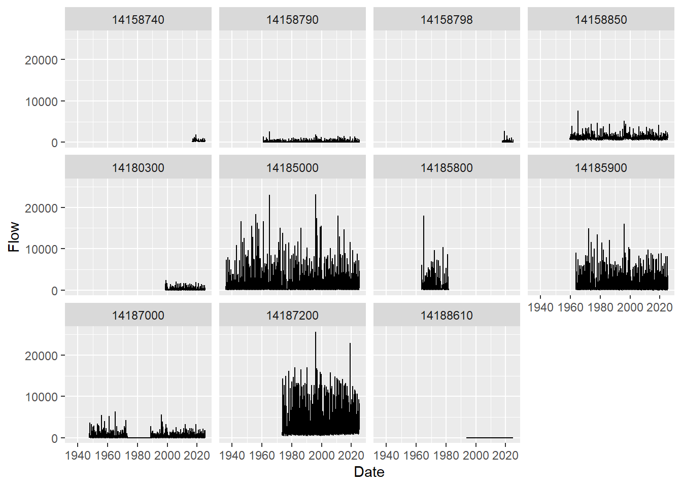
It looks like only 5 of our nwis sites had flow data for which we’ve plotted streamflow information for all the years available.
We’ve shown the client functionality for The Network-Linked Data Index (NLDI) using both nhdplusTools and dataRetrieval; either works similarly. The NLDI can index spatial and river network-linked data and navigate the river network to allow discovery of indexed information.
To use the NLDI you supply a starting feature which can be an:
- NHDPlus COMID
- NWIS ID
- WQP ID
- several other feature identifiers
You can see what is available with:
knitr::kable(dataRetrieval::get_nldi_sources())| source | sourceName | features |
|---|---|---|
| ca_gages | Streamgage catalog for CA SB19 | https://api.water.usgs.gov/nldi/linked-data/ca_gages |
| census2020-nhdpv2 | 2020 Census Block - NHDPlusV2 Catchment Intersections | https://api.water.usgs.gov/nldi/linked-data/census2020-nhdpv2 |
| epa_nrsa | EPA National Rivers and Streams Assessment | https://api.water.usgs.gov/nldi/linked-data/epa_nrsa |
| geoconnex-demo | geoconnex contribution demo sites | https://api.water.usgs.gov/nldi/linked-data/geoconnex-demo |
| gfv11_pois | USGS Geospatial Fabric V1.1 Points of Interest | https://api.water.usgs.gov/nldi/linked-data/gfv11_pois |
| GRAND | Selected GRAND Reservoirs | https://api.water.usgs.gov/nldi/linked-data/grand |
| HILARRI | HILARRI Hydropower Infrastructure | https://api.water.usgs.gov/nldi/linked-data/hilarri |
| huc12pp | HUC12 Pour Points NHDPlusV2 | https://api.water.usgs.gov/nldi/linked-data/huc12pp |
| huc12pp_102020 | HUC12 Pour Points circa 10-2020 | https://api.water.usgs.gov/nldi/linked-data/huc12pp_102020 |
| nmwdi-st | New Mexico Water Data Initative Sites | https://api.water.usgs.gov/nldi/linked-data/nmwdi-st |
| npdes | NPDES Facilities that Discharge to Water | https://api.water.usgs.gov/nldi/linked-data/npdes |
| nwisgw | NWIS Groundwater Sites | https://api.water.usgs.gov/nldi/linked-data/nwisgw |
| nwissite | NWIS Surface Water Sites | https://api.water.usgs.gov/nldi/linked-data/nwissite |
| ref_dams | geoconnex.us reference dams | https://api.water.usgs.gov/nldi/linked-data/ref_dams |
| ref_gage | geoconnex.us reference gages | https://api.water.usgs.gov/nldi/linked-data/ref_gage |
| vigil | Vigil Network Data | https://api.water.usgs.gov/nldi/linked-data/vigil |
| wade | Water Data Exchange 2.0 Sites | https://api.water.usgs.gov/nldi/linked-data/wade |
| wade_rights | Water Data Exchange Water Rights | https://api.water.usgs.gov/nldi/linked-data/wade_rights |
| wade_timeseries | Water Data Exchange Time Series | https://api.water.usgs.gov/nldi/linked-data/wade_timeseries |
| WQP | Water Quality Portal | https://api.water.usgs.gov/nldi/linked-data/wqp |
| comid | NHDPlus comid | https://api.water.usgs.gov/nldi/linked-data/comid |
4.2.2 Watershed data with StreamCatTools
StreamCatTools is an R package I’ve written that provides a client for the API for the StreamCat dataset, a comprehensive set of watershed data for the NHDPlus.
We can easily pull in watershed data from StreamCat for our basin with StreamCatTools:
comids <- SouthSantiam$UT_flowlines$nhdplus_comid
# we need a simple comma separated list for StreamCat
comids <- paste(comids,collapse=",",sep="")
df <- StreamCatTools::sc_get_data(metric='msst2014', aoi='other', comid=comids)
flowlines <- SouthSantiam$UT_flowlines
flowlines$msst2014 <- df$msst2014[match(flowlines$nhdplus_comid, df$comid)]
# drop any NAs
flowlines <- flowlines |> dplyr::filter(!is.na(flowlines$msst2014))
tm_shape(flowlines) + tm_lines("msst2014", title.col ="Mean Summer Stream\nTemperature (deg C) 2014") ── tmap v3 code detected ───────────────────────────────────────────────────────[v3->v4] `tm_lines()`: migrate the argument(s) related to the legend of the
visual variable `col` namely 'title.col' (rename to 'title') to 'col.legend =
tm_legend(<HERE>)'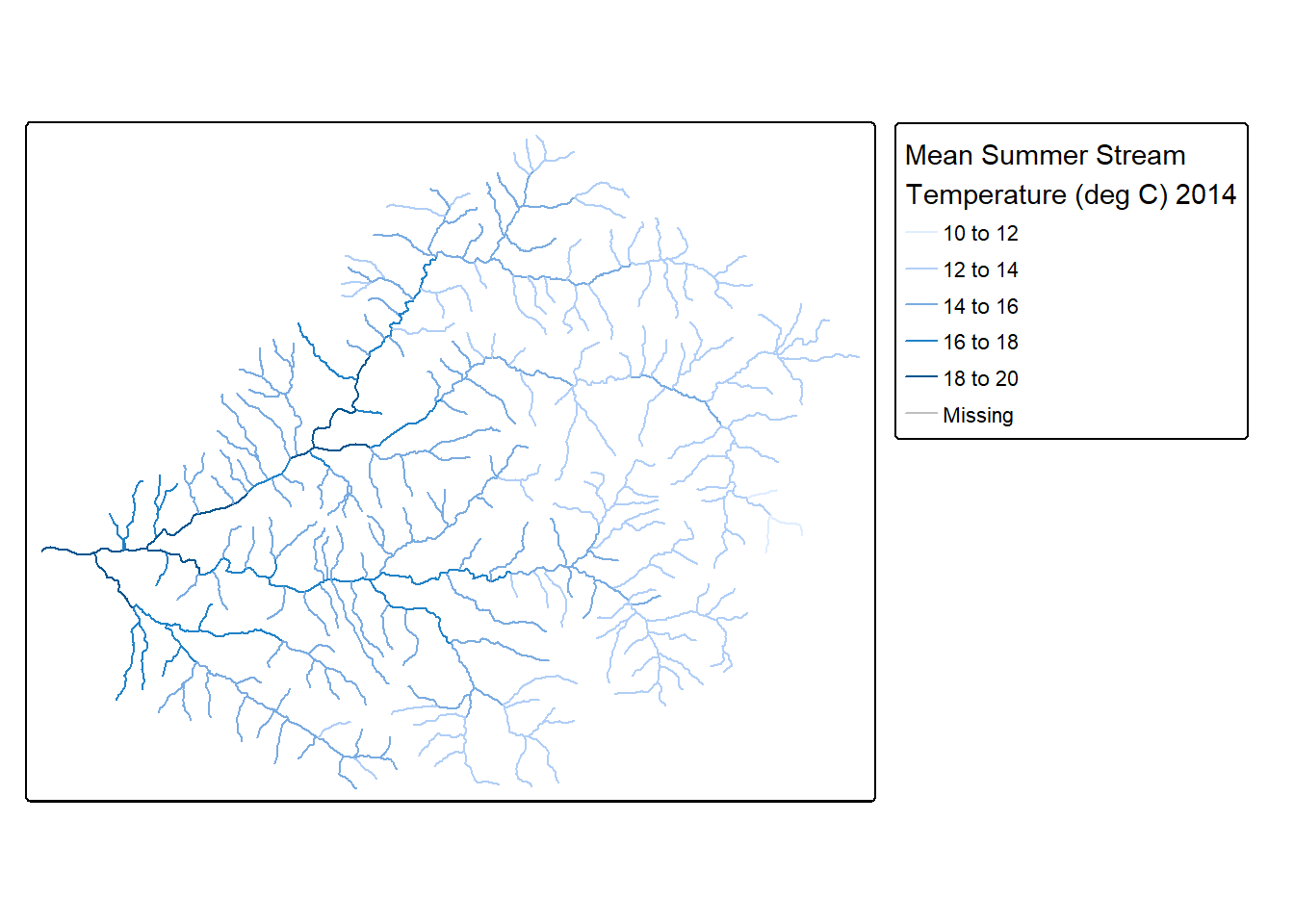
4.2.3 Elevation as a service
Thanks to our own Jeff Hollister we have the handy elevatr package for retrieving elevation data as a service for user provided points or areas - we can easily return elevation for our South Santiam basin we’ve created using elevation web services with elevatr:
elev <- elevatr::get_elev_raster(basin, z = 9)Mosaicing & ProjectingNote: Elevation units are in meters.mapview(elev)Warning in rasterCheckSize(x, maxpixels = maxpixels): maximum number of pixels for Raster* viewing is 5e+05 ;
the supplied Raster* has 991200
... decreasing Raster* resolution to 5e+05 pixels
to view full resolution set 'maxpixels = 991200 '4.2.4 OpenDAP and STAC
OPeNDAP allows us to access geographic or temporal slices of massive datasets over HTTP via web services. STAC similarly is a specification that allows us to access geospatial assets via web services. Using STAC you can access a massive trove of resources on Microsoft Planetary Computer via the rstac package as in examples here.
Here we’ll just show an example of using OpenDAP via Mike Johnson’s OpenDAP Catalog and ClimateR packages. Some of this from an Internet of Water webinar in 2022 with Mike Johnson and Taher Chagini
# See what is available - a LOT! As in 14,691 resources available via web services!!
dplyr::glimpse(opendap.catalog::params)Rows: 14,691
Columns: 15
$ id <chr> "hawaii_soest_1727_02e2_b48c", "hawaii_soest_1727_02e2_b48c"…
$ grid_id <chr> "73", "73", "73", "73", "73", "73", "73", "73", "73", "73", …
$ URL <chr> "https://apdrc.soest.hawaii.edu/erddap/griddap/hawaii_soest_…
$ tiled <chr> "", "", "", "", "", "", "", "", "", "", "", "", "", "", "", …
$ variable <chr> "nudp", "nusf", "nuvdp", "nuvsf", "nvdp", "nvsf", "sudp", "s…
$ varname <chr> "nudp", "nusf", "nuvdp", "nuvsf", "nvdp", "nvsf", "sudp", "s…
$ long_name <chr> "number of deep zonal velocity profiles", "number of surface…
$ units <chr> NA, NA, NA, NA, NA, NA, NA, NA, NA, NA, NA, NA, NA, NA, NA, …
$ model <chr> NA, NA, NA, NA, NA, NA, NA, NA, NA, NA, NA, NA, NA, NA, NA, …
$ ensemble <chr> NA, NA, NA, NA, NA, NA, NA, NA, NA, NA, NA, NA, NA, NA, NA, …
$ scenario <chr> NA, NA, NA, NA, NA, NA, NA, NA, NA, NA, NA, NA, NA, NA, NA, …
$ T_name <chr> "time", "time", "time", "time", "time", "time", "time", "tim…
$ duration <chr> "2001-01-01/2022-01-01", "2001-01-01/2022-01-01", "2001-01-0…
$ interval <chr> "365 days", "365 days", "365 days", "365 days", "365 days", …
$ nT <dbl> 22, 22, 22, 22, 22, 22, 22, 22, 22, 22, 22, 22, 22, 22, 22, …We can search for resources of interest:
opendap.catalog::search("monthly swe")# A tibble: 15 × 16
id grid_id URL tiled variable varname long_name units model ensemble
<chr> <chr> <chr> <chr> <chr> <chr> <chr> <chr> <chr> <chr>
1 GLDAS 139 http… "" swe_inst swe_in… "** snow… <NA> CLSM… <NA>
2 GLDAS 139 http… "" swe_inst swe_in… "** snow… <NA> CLSM… <NA>
3 GLDAS 135 http… "" swe_inst swe_in… "** snow… <NA> NOAH… <NA>
4 GLDAS 135 http… "" swe_inst swe_in… "** snow… <NA> NOAH… <NA>
5 GLDAS 139 http… "" swe_inst swe_in… "** snow… <NA> NOAH… <NA>
6 GLDAS 139 http… "" swe_inst swe_in… "** snow… <NA> NOAH… <NA>
7 GLDAS 139 http… "" swe_inst swe_in… "** snow… <NA> VIC10 <NA>
8 GLDAS 139 http… "" swe_inst swe_in… "** snow… <NA> VIC10 <NA>
9 NLDAS 174 http… "" swe swe "snow wa… kg m… MOS0… <NA>
10 NLDAS 174 http… "" swe swe "snow wa… kg m… NOAH… <NA>
11 NLDAS 174 http… "" swe swe "snow wa… kg m… VIC0… <NA>
12 terracli… 116 http… "" swe swe "snow_wa… mm <NA> <NA>
13 terracli… 116 http… "" swe swe "snow_wa… mm <NA> <NA>
14 terracli… 116 http… "" swe swe "snow_wa… mm <NA> <NA>
15 terracli… 116 http… "" swe swe "snow_wa… mm <NA> <NA>
# ℹ 6 more variables: scenario <chr>, T_name <chr>, duration <chr>,
# interval <chr>, nT <dbl>, rank <dbl>And we can extract a particular resource (in this case PRISM climate data) using climateR - we’ll go back to using our counties in Oregon data from earlier.
4.3 Transect example
d = dataRetrieval::findNLDI(location = c(-123.253375,44.553757), nav = "UM", find = c("flowlines", "basin"))
mapview(d, legend = FALSE)elev <- crop(
terra::rast("/vsicurl/http://mikejohnson51.github.io/opendap.catalog/ned_USGS_1.vrt"),
terra::vect(d$basin)
)
transect = extract(elev, vect(st_union(d$UM_flowlines))) |>
mutate(location = c(n():1))Warning: [extract] transforming vector data to the CRS of the rasterggplot(transect, aes(x = location, y = ned_USGS_1)) +
geom_line() +
geom_smooth()`geom_smooth()` using method = 'gam' and formula = 'y ~ s(x, bs = "cs")'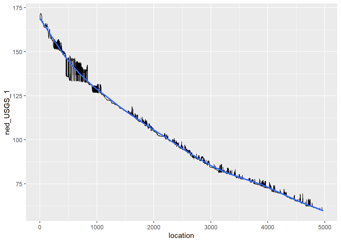
4.4 Geoconnex
Geoconnex builds and maintains the infrastructure and data needed to “make water data as easily discover-able, accessible, and usable as possible.”One of the datasets that this system has minted Persistent Identifiers (PIDs) for is a collection of USA mainstems. To be a “PID” a resource - in this case spatial feature - has to have a unique URI that can be resolved. This URI are store as JSON-LD, which, can be read by GDAL! So, if you can identify the geoconnex resource you want, you can read it into R and have confidence the URI will not change on you:
4.5 Zonal Statistics
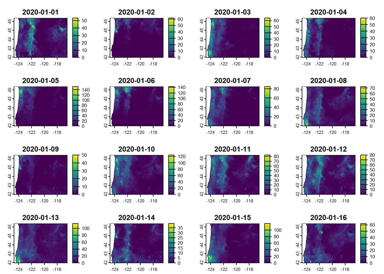
We can easily run zonal statistics for counties of Oregon using the zonal package with our precipitation data we extracted for Oregon from PRISM:
counties <- sf::st_transform(counties, crs(gridmet_or ))
county_precip <- zonal::execute_zonal(gridmet_or , counties, ID='name',fun='mean')
# Rename monthly precip
names(county_precip)[15:18] <- c('ppt_2020-01-01','ppt_2020-01-02',
'ppt_2020-01-03','ppt_2020-01-04')
a <- ggplot(county_precip, aes(fill=`ppt_2020-01-01`))+
geom_sf() +
scale_colour_gradientn(colours = terrain.colors(10))
b <- ggplot(county_precip, aes(fill=`ppt_2020-01-02`))+
geom_sf() +
scale_colour_gradientn(colours = terrain.colors(10))
c <- ggplot(county_precip, aes(fill=`ppt_2020-01-03`))+
geom_sf() +
scale_colour_gradientn(colours = terrain.colors(10))
d <- ggplot(county_precip, aes(fill=`ppt_2020-01-04`))+
geom_sf() +
scale_colour_gradientn(colours = terrain.colors(10))
plot_grid(a,b,c,d)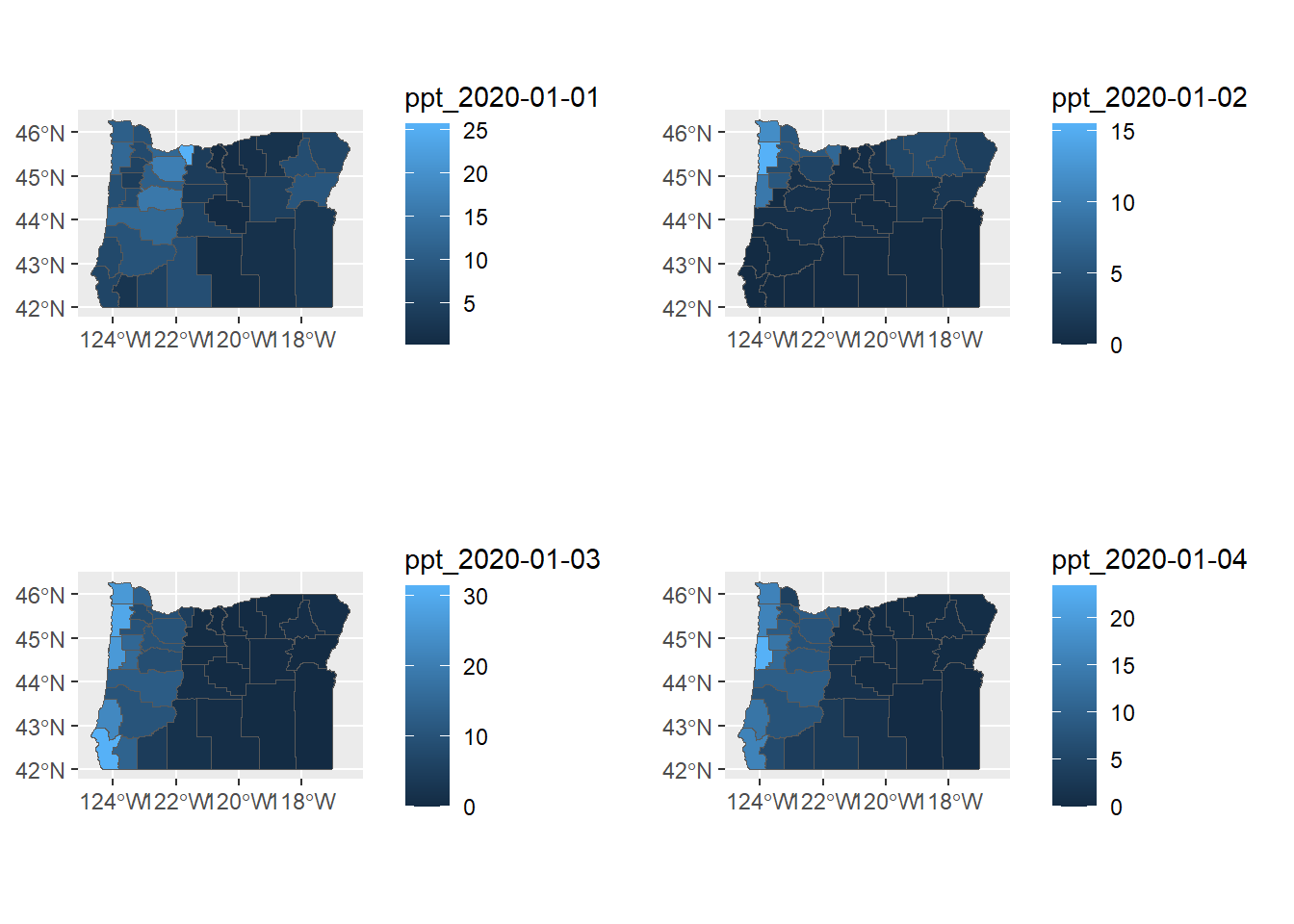
4.6 Extensions
4.6.1 RQGIS
There’s a bit of overhead to install QGIS and configure RQGIS - I use QGIS but have not set up RQGIS myself, I recommend reading the description in Geocomputation with R
4.6.2 R-ArcGIS bridge
See this description describing how to link your R install to the R-ArcGIS bridge
4.6.3 Accessing Python toolbox using reticulate
I highly recommend this approach if you want to integrate python workflows and libraries (including arcpy) with R workflows within reproducible R quarto or markdown files.
We can immediately start playing with python within a code block designated as python
import pandas as pd
print('hello python')
some_dict = {'a':1, 'b':2, 'c':3}
print(some_dict.keys())Load our gage data in Python…
import pandas as pd
gages = pd.read_csv('C:/Users/mweber/GitProjects/Rspatialworkshop/inst/extdata/Gages_flowdata.csv')
gages.head()
gages['STATE'].unique()
PNW_gages = gages[gages['STATE'].isin(['OR','WA','ID'])]4.6.3.1 Access Python objects directly from R
Now work with the pandas data directly within R
gages <- st_as_sf(py$PNW_gages,coords = c('LON_SITE','LAT_SITE'),crs = 4269)
gages <- st_transform(gages, crs=5070) #5070 is Albers system in metres
ggplot(gages) + geom_sf()And share spatial results from Python You can work with spatial tools in Python and share results with R!
from rasterstats import zonal_stats
clnp = 'C:/Users/mweber/Temp/CraterLake_tm.shp'
elev = 'C:/Users/mweber/Temp/elevation_tm.tif'
park_elev = zonal_stats(clnp, elev, all_touched=True,geojson_out=True, stats="count mean sum nodata")
geostats = gp.GeoDataFrame.from_features(park_elev)zonal <- py$geostats4.6.4 R Whitebox Tools
We won’t go into here but worth mentioning as a rich set of tools you can access in R - whiteboxR
4.6.5 rgee
Here I’m just running the demo code in the ReadMe for the rgee package as a proof of concept of cool things you can do being able to leverage Earth Engine directly in R. Note that there is overhead in getting this all set up.
library(reticulate)
library(rgee)
ee_Initialize()
# gm <- import("geemap")Function to create a time band containing image date as years since 1991.
createTimeBand <-function(img) {
year <- ee$Date(img$get('system:time_start'))$get('year')$subtract(1991L)
ee$Image(year)$byte()$addBands(img)
}Using Earth Engine syntax, we ‘Map’ the time band creation helper over the night-time lights collection.
collection <- ee$
ImageCollection('NOAA/DMSP-OLS/NIGHTTIME_LIGHTS')$
select('stable_lights')$
map(createTimeBand)We compute a linear fit over the series of values at each pixel, visualizing the y-intercept in green, and positive/negative slopes as red/blue.
col_reduce <- collection$reduce(ee$Reducer$linearFit())
col_reduce <- col_reduce$addBands(
col_reduce$select('scale'))
ee_print(col_reduce)We make an interactive visualization - pretty cool!