Lesson 1 - Spatial Data in R - sp
22 April 2018
So, to begin, what is R and why should we use R for spatial analysis? Let’s break that into two questions - first, what is R and why should we use it?
- A language and environment for statistical computing and graphics
- R is lightweight, free, open-source and cross-platform
- Works with contributed packages - currently 12,325 -extensibility
- Automation and recording of workflow (reproducibility)
- Optimized work flow - data manipulation, analysis and visualization all in one place
- R does not alter underlying data - manipulation and visualization in memory
- R is great for repetetive graphics
Second, why use R for spatial, or GIS, workflows?
- Spatial and statistical analysis in one environment
- Leverage statistical power of R (i.e. modeling spatial data, data visualization, statistical exploration)
- Can handle vector and raster data, as well as work with spatial databases and pretty much any data format spatial data comes in
- R’s GIS capabilities growing rapidly right now - new packages added monthly - currently about 180 spatial packages
Some drawbacks to using R for GIS work
- R not as good for interactive use as desktop GIS applications like ArcGIS or QGIS (i.e. editing features, panning, zooming, and analysis on selected subsets of features)
- Explicit coordinate system handling by the user, no on-the-fly projection support
- In memory analysis does not scale well with large GIS vector and tabular data
- Steep learning curve
- Up to you to find packages to do what you need - help not always great
An ideal solution for many tasks is using R in conjunction with traditional GIS software.
R runs on contributed packages - it has core functionality, but all the spatial work we would do in R is contained in user-contributed packages. Primary ones you’ll want to familiarize yourself with are sp, rgdal, sf, rgeos, raster - there are many, many more. A good source to learn about available R spatial packages is:
CRAN Task View: Analysis of Spatial Data
Lesson Goals
- Understanding of spatial data in R and
sp(spatial) objects in R - Introduction to R packages for spatial analysis
- Learn to read vector spatial data into
spobjects - Perform some simple exploratory spatial data analysis with vector data in R
Quick Links to Exercises and Material
- Exercise 1: Getting to Know of Spatial Objects
- Exercise 2: Building and Manipulating Spatial Data in R
- Exercise 3: Reading and writing data and projections
- Reading in Spatial Data: Reading in spatial data sets using rgdal
- R Spatial Resources
Download and extract data for exercises to your computer
download.file("https://github.com/mhweber/AWRA_GIS_R_Workshop/blob/gh-pages/files/SourceCode.R?raw=true",
              "SourceCode.R",
              method="auto",
              mode="wb")
download.file("https://github.com/mhweber/AWRA_GIS_R_Workshop/blob/gh-pages/files/WorkshopData.zip?raw=true",
              "WorkshopData.zip",
              method="auto",
              mode="wb")
download.file("https://github.com/mhweber/AWRA_GIS_R_Workshop/blob/gh-pages/files/HUCs.RData?raw=true",
              "HUCs.RData",
              method="auto",
              mode="wb")
download.file("https://github.com/mhweber/AWRA_GIS_R_Workshop/blob/gh-pages/files/NLCD_OR_2011.RData?raw=true",
              "NLCD_OR_2011.RData",
              method="auto",
              mode="wb")
unzip("WorkshopData.zip", exdir = ".")
A Little R Background
Terminology: Working Directory
Working directory in R is the location on your computer R is working from. To determine your working directory, in console type:
getwd()
Which should return something like:
[1] "/home/marc/GitProjects/AWRA_GIS_R_Workshop"
To see what is in the directory:
dir()
To establish a different directory:
setwd("/home/marc/GitProjects")
Terminology: data structures
R is an interpreted language (access through a command-line interpreter) with a number of data structures (vectors, matrices, arrays, data frames, lists) and extensible objects (regression models, time-series, geospatial coordinates) and supports procedural programming with functions.
To learn about objects, become friends with the built-in class and str functions. Let’s explore the built-in iris data set to start:
class(iris)
[1] "data.frame"
str(iris)
'data.frame':	150 obs. of  5 variables:
$ Sepal.Length: num  5.1 4.9 4.7 4.6 5 5.4 4.6 5 4.4 4.9 ...
$ Sepal.Width : num  3.5 3 3.2 3.1 3.6 3.9 3.4 3.4 2.9 3.1 ...
$ Petal.Length: num  1.4 1.4 1.3 1.5 1.4 1.7 1.4 1.5 1.4 1.5 ...
$ Petal.Width : num  0.2 0.2 0.2 0.2 0.2 0.4 0.3 0.2 0.2 0.1 ...
$ Species     : Factor w/ 3 levels "setosa","versicolor",..: 1 1 1 1 1 1 1 1 1 1 ...
As we can see, iris is a data frame and is used extensively for beginning tutorials on learning R. Data frames consist of rows of observations on columns of values for variables of interest - they are one of the fundamental and most important data structures in R.
But as we see in the result of str(iris) above, following the information that iris is a data frame with 150 observations of 5 variables, we get information on each of the variables, in this case that 4 are numeric and one is a factor with three levels.
First off, R has several main data types:
- logical
- integer
- double
- complex
- character
- raw
- list
- NULL
- closure (function)
- special
- builtin (basic functions and operators)
- environment
- S4 (some S4 objects)
- others you won’t run into at user level
We can ask what data type something is using typeof:
typeof(iris)
[1] "list"
typeof(iris$Sepal.Length)
[1] "double"
typeof(iris$Specis)
[1] "integer"
We see a couple interesting things here - iris, which we just said is a data frame, is a data type of list. Sepal.Length is data type double, and in str(iris) we saw it was numeric - that makes sense - but we see that Species is data type integer, and in str(iris) we were told this variable was a factor with three levels. What’s going on here?
First off, class refers to the abstract type of an object in R, whereas typeof or mode refer to how an object is stored in memory. So iris is an object of class data.frame, but it is stored in memory as a list (i.e. each column is an item in a list). Note that this allows data frames to have columns of different classes, whereas a matrix needs to be all of the same mode.
For our Species column, We see it’s mode is numeric, it’s typeof is integer, and it’s class is factor. Nominal variables in R are treated as a vector of integers 1:k, where k is the number of unique values of that nominal variable and a mapping of the character strings to these integer values.
This allows us to quickly see see all the unique values of a particular nominal variable or quickly re-asign a level of a nominal variable to a new value - remember, everything in R is in memory, so don’t worry about tweaking the data!
levels(iris$Species)
levels(iris$Species)[1] <- 'sibirica'
See if you can explain how that re-asignment we just did worked.
To access particular columns in a data frame, as we saw above, we use the $ operator - we can see the value for Species for each observation in `iris by doing:
iris$Species
To access particular columns or rows of a data frame, we use indexing:
iris[1,3] # the 1st row and the 3rd column
[1] 1.4
iris[4,5] # the 4th row and the 5th column
[1] sibirica
Levels: sibirica versicolor virginica
A handy function is names, which you can use to get or to set data frame variable names:
names(iris)
names(iris)[1] <- 'Length of Sepal'
Explain what this last line did
Overview of Classes and Methods
- Class: object types
class(): gives the class typetypeof(): information on how the object is storedstr(): how the object is structured
- Method: generic functions
print()plot()summary()
Exercise 1
Getting to Know of Spatial Objects
Handling of spatial data in R has been standardized in recent years through the base package sp - uses ‘new-style’ S4 classes in R that use formal class definitions and are closer to object-oriented systems than standard S3 classes in R.
The best source to learn about sp and fundamentals of spatial analysis in R is Roger Bivand’s book Applied Spatial Data Analysis in R
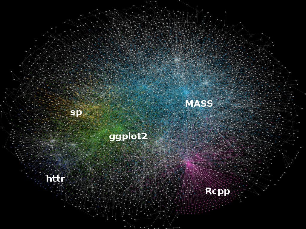
Although we’ll look at the new simple features object specification this morning as well, numerous packages are currently built using sp object structure so need to learn to navigate current R spatial ecosystem - image below from Colin Gillespie’s Tweet:
sp provides definitions for basic spatial classes (points, lines, polygons, pixels, and grids).
To start with, it’s good to stop and ask yourself what it takes to define spatial objects. What would we need to define vector (point, line, polygon) spatial objects?
- A coordinate reference system
- A bounding box, or extent
- plot order
- data
- ?
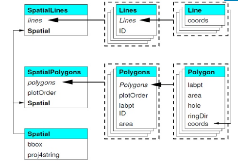
sp objects inherit from the basic spatial class, which has two ‘slots’ in R new-style class lingo. From the Bivand book above, here’s what this looks like (Blue at top of each box is the class name, items in white are the slots, arrows show inheritance between classes):
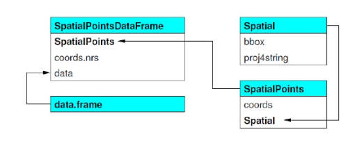
- Let’s explore this in R. We can use the
getClass()command to view the subclasses of a spatial object:
library(sp)
getClass("Spatial")
Class "Spatial" [package "sp"]

Slots:

Name:         bbox proj4string
Class:      matrix         CRS

Known Subclasses:
Class "SpatialPoints", directly
Class "SpatialGrid", directly
Class "SpatialLines", directly
Class "SpatialPolygons", directly
Class "SpatialPointsDataFrame", by class "SpatialPoints", distance 2
Class "SpatialPixels", by class "SpatialPoints", distance 2
Class "SpatialGridDataFrame", by class "SpatialGrid", distance 2
Class "SpatialLinesDataFrame", by class "SpatialLines", distance 2
Class "SpatialPixelsDataFrame", by class "SpatialPoints", distance 3
Class "SpatialPolygonsDataFrame", by class "SpatialPolygons", distance 2
Next we’ll delve a bit deeper into the spatial objects inhereting from the base spatial class and try creating some simple objects. Here’s a schematic of how spatial lines and polygons inherit from the base spatial class - again, from the Bivand book:
And to explore a bit in R:
getClass("SpatialPolygons")
Class "SpatialPolygons" [package "sp"]

Slots:

Name:     polygons   plotOrder        bbox proj4string
Class:        list     integer      matrix         CRS

Extends: "Spatial"

Known Subclasses:
Class "SpatialPolygonsDataFrame", directly, with explicit coerce
Also, there are a number of spatial methods you can use with classes in sp - here are some useful ones to familarize yourself with:
| Method / Class | Description |
|---|---|
| bbox() | Returns the bounding box coordinates |
| proj4string() | Sets or retrieves projection attributes using the CRS object |
| CRS() | Creates an object of class of coordinate reference system arguments |
| spplot() | Plots a separate map of all the attributes unless specified otherwise |
| coordinates() | Returns a matrix with the spatial coordinates. For spatial polygons it returns the centroids. |
| over(x, y) | Used for example to retrieve the polygon or grid indexes on a set of points |
| spsample(x) | Sampling of spatial points within the spatial extent of objects |
As an example data set to try out some of these methods on some spatial data in sp, we’ll load the nor2k data in the rgdal package which represents Norwegian peaks over 2000 meters:
library(rgdal)
data(nor2k)
plot(nor2k,axes=TRUE)
Take a few minutes to examine the nor2k SpatialPointsDataFrame and try using methods we’ve seen such as class(), str(), typeof(), proj4string(), etc.
A big part of working with spatial data in sp is understanding slots, and understanding how we access slots. The easiest way to access particular slots in an sp object is to use the @ symbol. You can also use the slotNames method. Take a few minutes using both to explore the structure of this simple sp object.
Exercise 2
Building and Manipulating Spatial Data in R
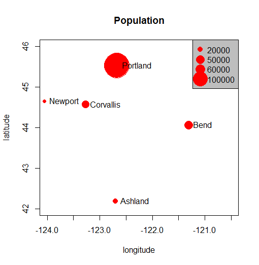
Let’s take a step back now. Basic data structures in R can represent spatial data - all we need is some vectors with location and attribute information
cities <- c('Ashland','Corvallis','Bend','Portland','Newport')
longitude <- c(-122.699, -123.275, -121.313, -122.670, -124.054)
latitude <- c(42.189, 44.57, 44.061, 45.523, 44.652)
population <- c(20062,50297,61362,537557,9603)
locs <- cbind(longitude, latitude)
plot(locs, cex=sqrt(population*.0002), pch=20, col='red',
  main='Population', xlim = c(-124,-120.5), ylim = c(42, 46))
text(locs, cities, pos=4)
Add a legend
breaks <- c(20000, 50000, 60000, 100000)
options(scipen=3)
legend("topright", legend=breaks, pch=20, pt.cex=1+breaks/20000,
  col='red', bg='gray')
Add a polygon to our map…
lon <- c(-123.5, -123.5, -122.5, -122.670, -123)
lat <- c(43, 45.5, 44, 43, 43)
x <- cbind(lon, lat)
polygon(x, border='blue')
lines(x, lwd=3, col='red')
points(x, cex=2, pch=20)
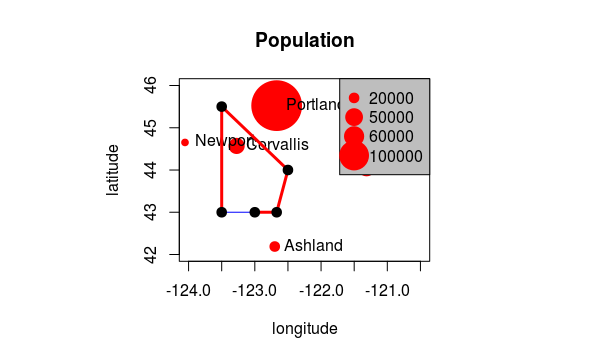
So, is this sufficient for working with spatial data in R and doing spatial analysis? What are we missing?
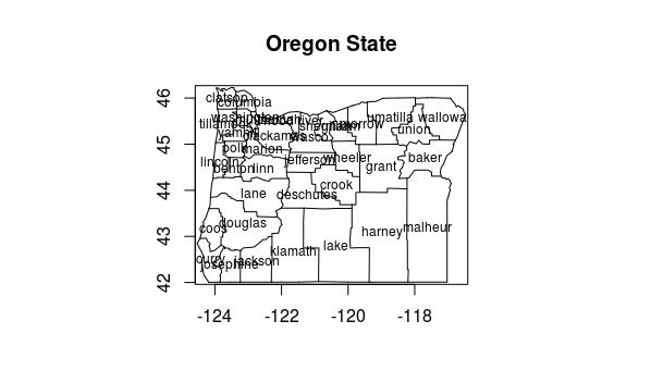
Packages early on in R came at handling spatial data in their own way. The maps package is great example - a database of locational information that is quite handy. The maps package format was developed in S (R is implementation of S) - lines represented as a sequence of points separated by ‘NA’ values - think of as drawing with a pen, raising at NA, then lowering at a value. Bad for associating with data since objects are only distinguished by separation with NA values. Try the following code-
library(maps)
map()
map.text('county','oregon')
map.axes()
title(main="Oregon State")
maps package draws on a binary database - see Becker references in help(map) for more details. Creates a list of 4 vectors when you create a maps object in R.
Explore the structure of map object a bit….
p <- map('county','oregon')
str(p)
p$names[1:10]
p$x[1:50]
Spatial classes provided in sp package have mostly standardized spatial data in R and provide a solid way to represent and work with spatial data in R.
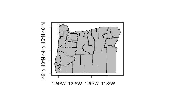
The maptools package provides convenience function for making spatial objects from map objects. Try the following code and see if you can follow each step…
library(maptools)
counties <- map('county','oregon', plot=F, col='transparent',fill=TRUE)
counties$names
#strip out just the county names from items in the names vector of counties
IDs <- sapply(strsplit(counties$names, ","), function(x) x[2])
counties_sp <- map2SpatialPolygons(counties, IDs=IDs,
    proj4string=CRS("+proj=longlat +ellps=WGS84 +datum=WGS84 +no_defs"))
summary(counties_sp)
plot(counties_sp, col="grey", axes=TRUE)
Exercise 3
Reading and writing data and projections
Now let’s look at how to construct a spatial object in R from a data frame with coordinate information.
StreamGages <- read.csv('StreamGages.csv')
class(StreamGages)
head(StreamGages)
A common GIS task you might do in R is taking a spreadsheet of data with coordinate information and turning it into a spatial object to do further GIS operations on. Here, we’ve read a speadsheet into an R data frame. Data frames, as we saw earlier, consist of rows of observations on columns of values for variables of interest
As with anything in R, there are several ways to go about this, but the basics are we need to pull the coordinate columns of the data frame into a matrix which becomes the coordinates slot of a spatial object, and then give the SpatialPointsDataFrame we create a coordinate reference system.
coordinates(StreamGages) <- c("LON_SITE","LAT_SITE")
proj4string(StreamGages) <- "+proj=longlat +datum=NAD83"
See how it looks
summary(StreamGages)
Object of class SpatialPointsDataFrame
Coordinates:
                min        max
LON_SITE -124.66912 -110.44111
LAT_SITE   41.42768   49.00075
Is projected: FALSE
proj4string :
[+proj=longlat +datum=NAD83 +ellps=GRS80 +towgs84=0,0,0]
Number of points: 2771
Data attributes:
   SOURCE_FEA             EVENTTYPE                                           STATION_NM       STATE
 Min.   :1.036e+07   StreamGage:2771   ABERDEEN-SPRINGFIELD CANAL NR SPRINGFIELD ID:   1   WA     :1054
 1st Qu.:1.233e+07                     ABERDEEN WASTE NR ABERDEEN ID               :   1   ID     : 800
 Median :1.307e+07                     ABERNATHY CREEK NEAR LONGVIEW, WA           :   1   OR     : 622
 Mean   :1.457e+07                     AENEAS LAKE NEAR TONASKET, WA               :   1   MT     : 220
 3rd Qu.:1.335e+07                     Agency Creek near Jocko MT (2)              :   1   WY     :  52
 Max.   :1.315e+09                     AGENCY CREEK NEAR JOCKO, MT                 :   1   NV     :  19
                                       (Other)                                     :2765   (Other):   4
Summary method gives a description of the spatial object in R. Summary works on pretty much all objects in R - for spatial data, gives us basic information about the projection, coordinates, and data for an sp object if it’s a spatial data frame object.
We can see the coordinate reference system information for our SpatialPointsDataFrame as part of output of summary, and we can also use the proj4string method to extract just this piece of information, or get the bounding box as well with bbox:
bbox(StreamGages)
proj4string(StreamGages)
Coordinate reference system, or CRS, information in sp uses the proj4string format. A very handy site to use to lookup any projection and get it’s proj4string format is spatialreference.org. A very handy resource put together by Melanie Frazier for an R spatial workshop we did several years ago, is here: Overview of Coordinate Reference Systems (CRS) in R.
A brief digression on CRS and projections in R
Dealing with coordinate reference systems and projections is a big part of working with spatial data in R, and it’s really relatively straightforward once you get the hang of it. Here are some of the fundamentals:
- CRS can be geographic (lat/lon), projected, or NA in R
- Data with different CRS MUST be transformed to common CRS in R
- Projections in
spare provided in PROJ4 strings in the proj4string slot of an object - http://www.spatialreference.org/
- Useful
rgdalpackage functions:- projInfo(type=’datum’)
- projInfo(type=’ellps’)
- projInfo(type=’proj’)
- For
spclass objects:- To get the CRS: proj4string(x)
- To assign the CRS:
- Use either EPSG code or PROJ.4:
- proj4string(x) <- CRS(“+init=epsg:4269”)
- proj4string(x) <- CRS(“+proj=utm +zone=10 +datum=WGS84”)
- Use either EPSG code or PROJ.4:
- To transform CRS
- x <- spTransform(x, CRS(“+init=epsg:4238”))
- x <- spTransform(x, proj4string(y))
- For rasters (we’ll focus on rasters later, but mention projections here):
- To get the CRS: projection(x)
- To transform CRS: projectRaster(x)
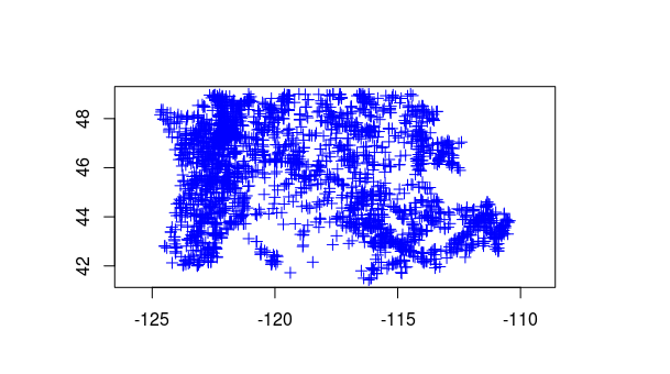
We can use the generic plot function in R to produce a quick plot as well as add axes - axes option puts box around region
plot(StreamGages, axes=TRUE, col='blue')
And we can combine and use state borders from maps package in our map
map('state',regions=c('oregon','washington','idaho'),fill=FALSE, add=T)

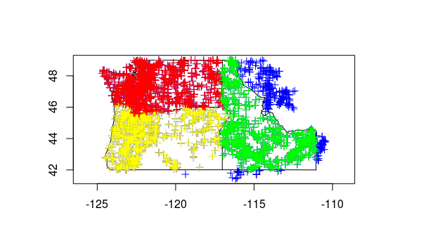
We can also use subsetting with plotting with this stream gage data to symbolize our gages by state for instance - try the following lines, try different colors or border states
plot(StreamGages[StreamGages$STATE=='OR',],add=TRUE,col="Yellow") #plot just the Oregon sites in yellow on top of other sites
plot(StreamGages[StreamGages$STATE=='WA',],add=TRUE,col="Red")
plot(StreamGages[StreamGages$STATE=='ID',],add=TRUE,col="Green")
Now let’s load the Rdata object we downloaded at beginning of this session - Rdata files are just a handy way of saving and reloading your workspace - remember, R works with objects in memory, you can save them out in this format or share with others this way.
Let’s look at a SptialPolygonsDataframe of HUCs and dig into slot structure for polygon data in sp. For a more complex object like a SptialPolygonsDataframe there is a hierarchy of slots we need to understand.
load("HUCs.RData")
class(HUCs)
getClass("SpatialPolygonsDataFrame")
summary(HUCs)
slotNames(HUCs) #get slots using method
str(HUCs, 2)
head(HUCs@data) #the data frame slot
HUCs@bbox #call on slot to get bbox
Try to figure out what the following lines of code doing - welcome to the wonderful world of slots in R. Take a minute to look at and run examples at bottom of help when you run help(slotNames) - it will help make more sense of things.
# Each polygon element has 5 of it's own slots:
HUCs@polygons[[1]]
slotNames(HUCs@polygons[[1]])
HUCs@polygons[[1]]@labpt
# This is how we access the area of the first feature in HUCs
HUCs@polygons[[1]]@Polygons[[1]]@area
What are the slots within each element of the HUCs SpatialPolygonDataFrame object polygons slot?
What method do you use to list them?
What is the length of HUCs@polygons?
Note that we can also make use of the gArea function in the rgeos package. gArea expects a planar CRS, so let’s transform to Oregon Lambert, but let’ use the epsg code (which we can look up on spatialreference.org) rather than passing a projection string to spTransform:
library(rgeos)
HUCs <- spTransform(HUCs,CRS("+init=epsg:2991"))
gArea(HUCs) #Total area of all features
gArea(HUCs[1,]) # Area of the first feature, equivalent to:
HUCs@polygons[[1]]@area
gArea(HUCs[2,]) # Area of the second feature, equivalent to:
HUCs@polygons[[2]]@area
How would we code a way to extract the HUCs polygon with the smallest area? Hint - apply family of functions and slots - try on your own and then take a look at the function that I included as part of HUCs.RData file. Many of you are likely not familiar with the apply family of functions in R - it is well worth getting to know them. This answer to a question on Stackoverflow is a fanctastic description.
Spatial Overlay
Using the over function, we can find out what HUC every stream gage is in quite easily:
StreamGages <- spTransform(StreamGages, CRS(proj4string(HUCs)))
gage_HUC <- over(StreamGages,HUCs, df=TRUE)
# We have a data frame of results, next we match it back to our StreaGages
StreamGages$HUC <- gage_HUC$HUC_8[match(row.names(StreamGages),row.names(gage_HUC))]
head(StreamGages@data)
There’s a fair bit to unpack there, so ask questions!
Joining
We can join tabular attributes to our spatial data - let’s say we have flow data for our gages we want to join
gage_flow <- read.csv("Gages_flowdata.csv")
StreamGages$AVE <- gage_flow$AVE[match(StreamGages$SOURCE_FEA,gage_flow$SOURCE_FEA)] # add a field for average flow
Overlay and aggregation
We can use over to do a summary like ‘calculate the average flow within all HUCs of the gage average stream flows’ or get total flow - look at head of the two results:
HUC.Flow <- over(HUCs,StreamGages[5],fn = mean)
HUC.Flow <- over(HUCs,StreamGages[5],fn = sum)
See the SourceCode.R file if you want for an extra example of performing a dissolve operation on the HUCS data.
Reading in Spatial Data
You’ll typically want to read and write shapefiles and geodatabase features when working in R - rgdal is the workhorse for this. To see what vector data formats you can read / write using rdal, type:
ogrDrivers()
You have tons of options available! Here are a couple quick examples for both shapefile and geodatabase features using rgdal (replace my example file paths with file paths to use to working directory on your computer:
Reading in shapefiles:
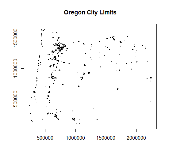
download.file("ftp://ftp.gis.oregon.gov/adminbound/citylim_2017.zip","citylim_2017.zip")
unzip("citylim_2017.zip", exdir = ".")
citylims <- readOGR(".", "citylim_2017") # our first parameter is directory, in this case '.' for working directory, and no extension on file!
plot(citylims, axes=T, main='Oregon City Limits') # plot it!
Reading in geodatabases:
# Geodatabase Example
download.file("https://www.blm.gov/or/gis/files/web_corp/state_county_boundary.zip","state_county_boundary.zip")
unzip("state_county_boundary.zip", exdir = "/home/marc")
fgdb = "state_county_boundary.gdb"

# List all feature classes in a file geodatabase
fc_list = ogrListLayers(fgdb)
print(fc_list)
##[1] "state_poly" "cob_poly"   "cob_arc"
##attr(,"driver")
##[1] "OpenFileGDB"
##attr(,"nlayers")
##[1] 3
# Read the feature class
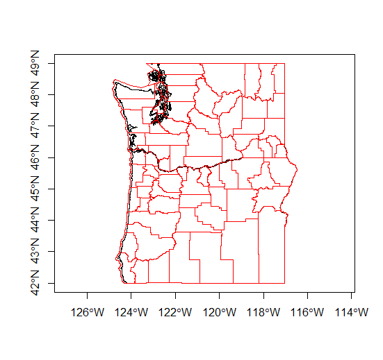
state_poly = readOGR(dsn=fgdb,layer="state_poly")
plot(state_poly, axes=TRUE)
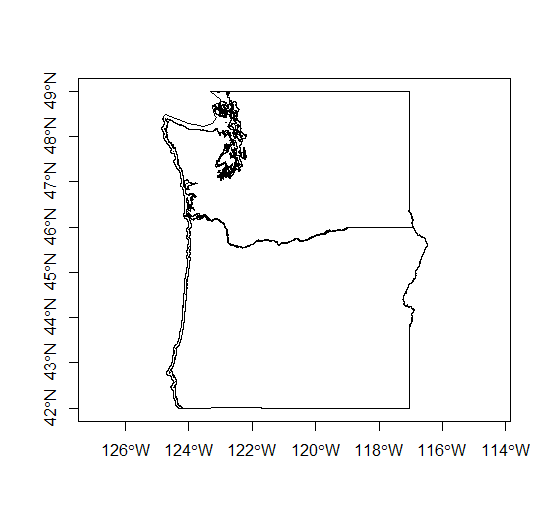
cob_poly = readOGR(dsn=fgdb,layer="cob_poly")
plot(cob_poly, add=TRUE, border='red')