Lesson 2 - Spatial Data in R - sf
22 April 2018
The sf Simple Features for R package by Edzer Pebesma is a move from the sp S4 or new style class representation of spatial data in R, and instead provides simple features access for R. Without a doubt, sf will replace sp as the fundamental spatial model in R for vector data - packages are already being updated around sf, and it fits in with the “tidy” approach to data of Hadley Wickham’s tidyverse. The simple feature model will be familiar to folks who use PostGIS, MySQL Spatial Extensions, Oracle Spatial, the OGR component of the GDAL library, GeoJSON and GeoPandas in Python. Simple features are represented with Well-Known text - WKT - and well-known binary formats.
The big difference is the use of S3 classes in R rather than the S4, or new style classes, used in sp with the use of slots. Simple features are simply data.frame objects that have a geometry list-column. sf interfaces with GEOS for topolgoical operations, uses GDAL for data creation and I/O, and can directly read and write to spatial databases such as PostGIS. Additionally, as mentioned above, sf fits into the tidyverse design, and the list-column for geometry are officially considered a tidy data form. See Edzer Pebesma’s Spatial Data in R: New Directions post for the description of tidy aspects of sf.
Just as in PostGIS, all functions and methods in sf are prefixed with st_, which stands for ‘spatial and temporal’. An advantage of this prefixing is all commands are easy to find with command-line completion in sf.
Edzar Pebesma has extensive documentation, blog posts and vignettes available for sf here:
Simple Features for R. Additionally, see Edzar’s r-spatial blog which has numerous announcements, discussion pieces and tutorials on spatial work in R focused.
Lesson Goals
- Learn the structure of
sfobjects using some example water sample data - Understand plotting with of
sfobjects - Use topological operations in
sfsuch as spatial intersections, joins and aggregations with example data
Quick Links to Exercises
- Exercise 1: Getting to Know
sf - Exercise 2: Spatial operations - spatial subsetting and intersecting
- Exercise 3: Spatial operations - joins
- Exercise 4: Spatial operations - aggregation
- Reading in Spatial Data with
sf: Reading in spatial data sets using rgdal - R
sfResources
First, if not already installed, install sf. You can either install from CRAN or you can install the most current development version from Github - both methods shown below.
# From CRAN:
install.packages("sf")
# From GitHub:
library(devtools)
# install_github("edzer/sfr")
library(sf)
## Linking to GEOS 3.5.0, GDAL 2.1.1, proj.4 4.9.3
The sf package has numerous topological methods for performing spatial operations.
methods(class = "sf")
[1] [                 aggregate         cbind
[4] coerce            initialize        plot
[7] print             rbind             show
[10] slotsFromS3       st_agr            st_agr<-
[13] st_as_sf          st_bbox           st_boundary
[16] st_buffer         st_cast           st_centroid
[19] st_convex_hull    st_crs            st_crs<-
[22] st_difference     st_drop_zm        st_geometry
[25] st_geometry<-     st_intersection   st_is
[28] st_linemerge      st_polygonize     st_precision
[31] st_segmentize     st_simplify       st_sym_difference
[34] st_transform      st_triangulate    st_union
see '?methods' for accessing help and source code
Exercise 1
Getting to Know sf
To begin exploring, let’s read in some spatial data. We’ll grab EPA Wadeable Streams Assessment sites to begin looking at.
library(RCurl)
library(sf)
library(ggplot2)
library(dplyr)
download <- getURL("https://www.epa.gov/sites/production/files/2014-10/wsa_siteinfo_ts_final.csv")

wsa <- read.csv(text = download)
class(wsa)
Just a data frame that includes location and other identifying information about river and stream sampled sites from 2000 to 2004.
[1] "data.frame"
Before we go any further, let’s subset our data to just the US plains ecoregions using the ‘ECOWSA9’ variable in the wsa dataset.
levels(wsa$ECOWSA9)
wsa_plains <- wsa[wsa$ECOWSA9 %in% c("TPL","NPL","SPL"),]
And now that we’ve done this subsetting, I want to show you how to do another way using the dplyr package.
Remember at the beginning I said one of the advantages of sf is that it fits into the tidyverse way of operating and really streamlines our ability to work with spatial data in R. One concrete example, which we’ll build on in this section, is that we can manipulate and reshape sf spatial data directly using dplyr and tidyr verbs.
Let’s do the same subsetting step above using dplyr - for some of you this will be familiar territory, for others it may be confusing - the idea with dplyr and ‘chained’ operations is that it allows you to do more expressive sequences of operations on data in the order you typically think about doing it, rather than created convoluted nested statements in R.
wsa_plains <- wsa %>%
  # select a just the plains states using dplyr::filter
  dplyr::filter(ECOWSA9 %in% c("TPL","NPL","SPL"))
dplyr
In this section we’ll use dplyr several times, so let’s just review the ‘verbs’ in dplyr - these methods operate just on the attribute data in our sf data frame and leave the geometries untouched.
- select() keeps only certain variables
- rename() renames a variable and leaves all others unchanged
- filter() returns rows that match a certain condition(s)
- mutate() adds new variables based on existing variables
- transmute() creates new variables and drops existing variables
- arrange() sorts the data frame the by a variable(s)
- slice() selects rows based on row number
- sample_n() samples n features randomly
Others, such as summarise, will actually aggregate (union) underlying geometry - again, see Edzer Pebesma’s Spatial Data in R: New Directions post at end for details.
Because both the wsa and wsa_plains dataframes have coordinate information, we can then promotote either of them to an sf spatial object.
wsa_plains = st_as_sf(wsa_plains, coords = c("LON_DD", "LAT_DD"), crs = 4269,agr = "constant")
str(wsa_plains)
Note that this is now still a dataframe but with an additional geometry column. sf objects are still a data frame, but have an additional list-column for geometry.
What is different about an sf dataframe, and what is code below doing?
head(wsa_plains[,c(1,60)])
Simple feature collection with 6 features and 1 field
Attribute-geometry relationship: 1 constant, 0 aggregate, 0 identity
geometry type:  POINT
dimension:      XY
bbox:           xmin: -104.7643 ymin: 39.35901 xmax: -91.92294 ymax: 42.70254
epsg (SRID):    4269
proj4string:    +proj=longlat +ellps=GRS80 +towgs84=0,0,0,0,0,0,0 +no_defs
        SITE_ID                    geometry
13        CC0001  POINT(-104.76432 39.35901)
14 IAW02344-0096 POINT(-94.089731 41.950878)
15 IAW02344-0096 POINT(-94.089731 41.950878)
16 IAW02344-0097 POINT(-95.400885 41.332723)
17 IAW02344-0097 POINT(-95.400885 41.332723)
18 IAW02344-0098   POINT(-91.92294 42.70254)
We can do simple plotting just as with sp spatial objects. sf by default creates a multi-panel lattice plot much like the sp package spplot function - either plot particular columns in multiple plots or specify the geometry column to make a single simple plot. Note how it’s easy to use graticules as a parameter for plot in sf.
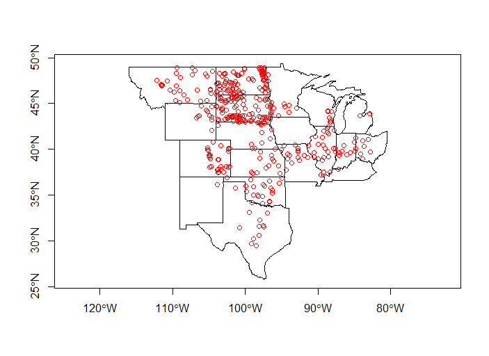
plot(wsa_plains[c(46,56)], graticule = st_crs(wsa_plains), axes=TRUE)
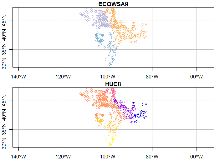
Try some of these variations and see if they make sense to you.
plot(wsa_plains[c(38,46)],graticule = st_crs(wsa_plains), axes=TRUE)
plot(wsa_plains['geometry'], main='Keeping things simple',graticule = st_crs(wsa_plains), axes=TRUE)
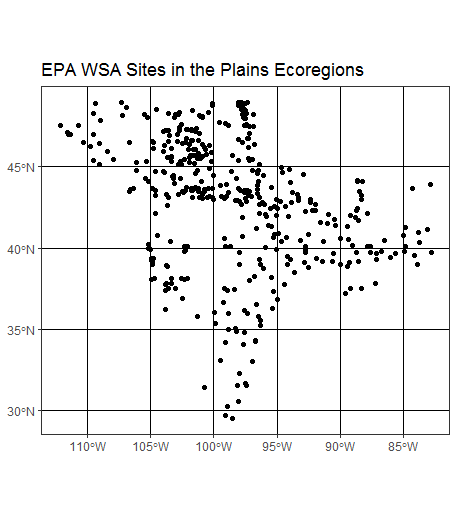
And ggplot2 now supports directly plotting sf features using sf_geom - another step forward in streamling our work with spatial data in sf:
ggplot(wsa_plains) +
  geom_sf() +
  ggtitle("EPA WSA Sites in the Plains Ecoregions") +
  theme_bw()
A quick note on converting between sp and sf
Converstion to and from sp and sf is quite easy (in principle!), example with our nor2k data:
class(nor2k)
nor2k_sf <- st_as_sf(nor2k)
Error: is.numeric(bb) && length(bb) == 4 is not TRUE
Wait a minute, I just said it was easy - why are we getting this error? This is a typical example of working in R - the thing you’re trying to do ends up being the exception to the rule! Take a minute and see if you can figure out why we’re getting this problem and what we need to do to fix it - answer is in SourceCode.R. Once converted, let’s convert it back to an sp SpatialPointsDataFrame.
class(nor2k_sf)
nor2k_sp <- as(nor2k_sf, "Spatial")
class(nor2k_sp)
See sp-sf Migration also listed at end of this section under R sf Resources for table of equivalent sf commands for sp commands (as well as sf equivalents for rgeos and rgdal commands)
Exercise 2
Spatial operations - spatial subsetting and intersecting
Now let’s grab some administrative boundary data, for instance US states. After bringing in, let’s examine the coordinate system and compare with the coordinate system of the WSA data we already have loaded. Remember, in sf, as with sp, we need to have data in the same CRS in order to do any kind of spatial operations involving both datasets.
library(sf)
library(USAboundaries)
states  <- us_states()
levels(as.factor(states$state_abbr))
states <- states[!states$state_abbr %in% c('AK','PR','HI'),]

st_crs(states)
st_crs(wsa_plains)
They’re not equal, which we verify with:
st_crs(states) == st_crs(wsa_plains)
We’ll tranfsorm the WSA sites to same CRS as states
wsa_plains <- st_transform(wsa_plains, st_crs(states))
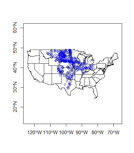
Now we can plot together in base R
plot(states$geometry, axes=TRUE)
plot(wsa_plains$geometry, col='blue',add=TRUE)
Quick exercise - sf geometry
As I mentioned earlier, feature geometry in sf is a list-column.
We access the geometry column using: states$geometry
We know each element in the column is a list.
The geometry column is presented as well-known text, in the form of: Multipolygon(polygon1, polygon2).
polygon1 might have 1 more holes, and could be represented itself as (poly1, hole1, hole2).
Each polygon and it’s holes are held together by a set of parantheses, so: Multipolygon(((polygon1))) indicates the exterior ring coordinates, without holes, of the first polygonn.
See Edzer’s simple feature geometry list-column explanation for more details.
Knowing all this, see if you can figure out how we would:
- Show the geometry of the first multipolygon feature in states
- Show the coordinates of the 1st polygon of the first multipolygon in states
- Show the first 3 coordinate pairs of the first polygon of the second multi-polygon feature in states
- Plot just the first multipolygon feature in states
Spatial subsetting
Spatial subsetting is an essential spatial task and can be performed just like attribute subsetting in sf. Say we want to pull out just the states that intersect our ‘wsa_plains’ sites that we’ve subset via an attribute query - it’s as simple as:
plains_states <- states[wsa_plains,]
There are actually several ways to achieve the same thing - here’s another:
plains_states <- states[wsa_plains,op = st_intersects]
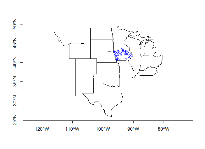
And we can do another attribute subset and then apply a spatial subset yet another way - verify this works for you by plotting results together
iowa = states[states$state_abbr=='IA',]
iowa_sites <- st_intersection(wsa_plains, iowa)
It’s worth spending some time with the topological operations in sf. st_intersection as used above returns an sf data frame of the wsa_plains sites that intersect the iowa polygon. st_intersects on the other hand returns either a list or matrix of true / false values - for instance:
sel_list <- st_intersects(wsa_plains, iowa)
This first selection returns a list with a positive (1) value where there is an intersection and empty result where no intersection
This second selection below returns a matrix of true / false values for intersections and can be used for subsetting the original data
sel_mat <- st_intersects(wsa_plains, iowa, sparse = FALSE)
iowa_sites <- wsa_plains[sel_mat,]
plot(plains_states$geometry, axes=T)
plot(iowa_sites, add=T, col='blue')
What about all our sites that are not in Iowa?
sel_mat <- st_disjoint(wsa_plains, iowa, sparse = FALSE)
not_iowa_sites <- wsa_plains[sel_mat,]
plot(plains_states$geometry, axes=T)
plot(not_iowa_sites, add=T, col='red')
Exercise 3
Spatial operations - joins
Spatial joining in R is an incredibly handy thing and is simple with st_joins. Many of us are likely old hands at doing attribute joins of shapefiles with other tabular data in GIS software like ArcGIS or QGis.
By default st_joins will perform a left join (return all rows in the left, ‘joined to’ table regardless of whether there are matches in the right, ‘joined’ table). st_joins also uses st_intersect for the spatial operation. Note that you can also do an inner join (a match in both tables) as well as use other topological operations for the join such as st_touches, st_disjoint, st_equals, etc.
For this simple example, we’ll strip out the state and most other attributes from our WSA sites we’ve been using, and then use the states sf file in a spatial join to get state for each site spatially. This is a typical task many of us frequently face - assign attribute information from some spatial unit for points within the unit.
So we’re asking, in code below, “what state is each WSA site in?”, based on where it is located.
# Use column indexing to subset just a couple attribute columns - need to keep geometry column!
wsa_plains <- wsa_plains[c(1:4,60)]
wsa_plains <- st_join(wsa_plains, plains_states)
# verify your results
head(wsa_plains)
simple feature collection with 6 features and 16 fields
geometry type:  POINT
dimension:      XY
bbox:           xmin: -104.7643 ymin: 39.35901 xmax: -91.92294 ymax: 42.70254
epsg (SRID):    4326
proj4string:    +proj=longlat +datum=WGS84 +no_defs
         SITE_ID YEAR VISIT_NO               SITENAME statefp  statens    affgeoid geoid stusps     name lsad        aland
13        CC0001 2004        1           CHERRY CREEK      08 01779779 0400000US08    08     CO Colorado   00 268429343790
14 IAW02344-0096 2004        1          BEAVER BRANCH      19 01779785 0400000US19    19     IA     Iowa   00 144667643793
15 IAW02344-0096 2004        2          BEAVER BRANCH      19 01779785 0400000US19    19     IA     Iowa   00 144667643793
16 IAW02344-0097 2004        1 WEST NISHNABOTNA RIVER      19 01779785 0400000US19    19     IA     Iowa   00 144667643793
17 IAW02344-0097 2004        2       WEST NISHNABOTNA      19 01779785 0400000US19    19     IA     Iowa   00 144667643793
18 IAW02344-0098 2004        1  UNN TRIB. OTTER CREEK      19 01779785 0400000US19    19     IA     Iowa   00 144667643793
       awater state_name state_abbr jurisdiction_type                   geometry
13 1175112870   Colorado         CO             state POINT (-104.7643 39.35901)
14 1077808017       Iowa         IA             state POINT (-94.08973 41.95088)
15 1077808017       Iowa         IA             state POINT (-94.08973 41.95088)
16 1077808017       Iowa         IA             state POINT (-95.40089 41.33272)
17 1077808017       Iowa         IA             state POINT (-95.40089 41.33272)
18 1077808017       Iowa         IA             state POINT (-91.92294 42.70254)
Let’s dive a little deeper with spatial joins and bring in some water quality data using the dataRetrieval package to access data via web services on the Water Quality Portal. Steps shown here follow examples in the tutorial.
First we’ll load the dataRetrieval library and pull down some nitrogen data for Iowa to play with. Note how we pull out siteInfo below - this is a data table attribute of distinct sites in the IowaNitrogen object pulled down - explore the object a bit (using str or class or other means).
library(dataRetrieval)
IowaNitrogen<- readWQPdata(statecode='IA', characteristicName="Nitrogen")
head(IowaNitrogen)
names(IowaNitrogen)

siteInfo <- attr(IowaNitrogen, "siteInfo")
unique(IowaNitrogen$ResultMeasure.MeasureUnitCode)
Next we need to take this raw data and do some filtering and summarizing to get data we can use for mapping and joining with the WSA data we’ve been using so far. Spend a little time and see if you can follow what we’re doing below - notice the way the dplyr functions are being called here - why might that be needed as oppossed to typical way of calling functions? Take a few minutes and try to follow what each of the chained operations are doing on this Iowa nitrogen data.
IowaSummary <- IowaNitrogen %>%
  dplyr::filter(ResultMeasure.MeasureUnitCode %in% c("mg/l","mg/l      ")) %>%
  dplyr::group_by(MonitoringLocationIdentifier) %>%
  dplyr::summarise(count=n(),
            start=min(ActivityStartDateTime),
            end=max(ActivityStartDateTime),
            mean = mean(ResultMeasureValue, na.rm = TRUE)) %>%
  dplyr::arrange(-count) %>%
  dplyr::left_join(siteInfo, by = "MonitoringLocationIdentifier")
Now we just need to make the data spatial - we have coordinates so it’s as simple as:
iowa_wq = st_as_sf(IowaSummary, coords = c("dec_lon_va", "dec_lat_va"), crs = 4269,agr = "constant")
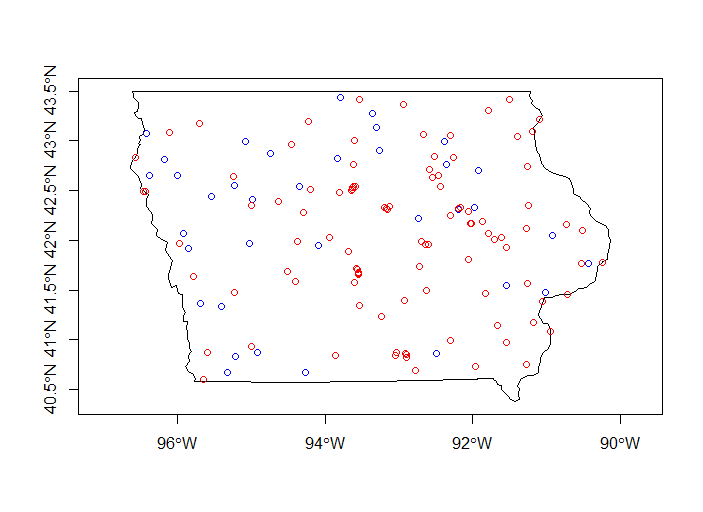
Let’s plot it with our other data and see what we’ve got - tip for subsetting while plotting is from rpubs here.
plot(st_geometry(subset(states, state_abbr == 'IA')), axes=T)
plot(st_geometry(subset(wsa_plains, stusps =='IA')), add=T, col='blue')
plot(iowa_wq, add=T, col='red')
Proximity analysis
Now let’s try to join this water quality nitrogen data in a given proximity to WSA sampled sites. We’ll first need to transform the data to a projected coordinate system since we’ll be using distance in our join this time. sf can make use of both proj4 strings and epsg codes - to find the epsg code for UTM zone 15 in Iowa which we’re using here just search on spatialreference.org. Note our projection is in meters so we set our distance very high - obviously we wouldn’t join water quality sites tens to hundreds of kilometers away to other sites using euclidean distance for a real application - this is just for illustrative purposes to show how we can do distance based joins in sf.
wsa_iowa <- subset(wsa_plains, state_abbr=='IA')
wsa_iowa <- st_transform(wsa_iowa, crs=26915)
iowa_wq <- st_transform(iowa_wq, crs=26915)

wsa_wq = st_join(wsa_iowa, iowa_wq, st_is_within_distance, dist = 50000)
You’ll see if you do head on your data there are a LOT of fields in there now - what we’re interested in is the mean field we calcluated earlier in dplyr steps that gives us mean nitrogren concentration at water quality sites.
Exercise 4
Spatial operations - aggregation
Now that we’ve joined water quality data based on proximity to our WSA sample sites, we can aggregate the results for each WSA site.
What happened in the previous spatial join step we performed was that we generated a new record for every water quality site within the proximity we gave to our WSA sites - check the number of records in the wsa_iowa data versus the number of records in our join result - we haved repeated records for unique WSA sites.
So let’s aggregate results using dplyr - take a few minutes and see if you can figure out how on your own! The answer is in the SourceCode.R file, but try a bit on your own first, and then if needed run and try to follow the anwer code in SourceCode.R file.
For performing spatial aggregation, the idea is to take some spatial data, and summarize that data in relation to another spatial grouping variable (think city populations averaged by state). Using some of the data we’ve used in previous steps, we can accomplish this in a couple of ways.
Let’s grab some chemistry data for the WSA sites we’ve been using so far:
download <- getURL("https://www.epa.gov/sites/production/files/2014-10/waterchemistry.csv")

wsa_chem <- read.csv(text = download)
wsa$COND <- wsa_chem$COND[match(wsa$SITE_ID, wsa_chem$SITE_ID)]
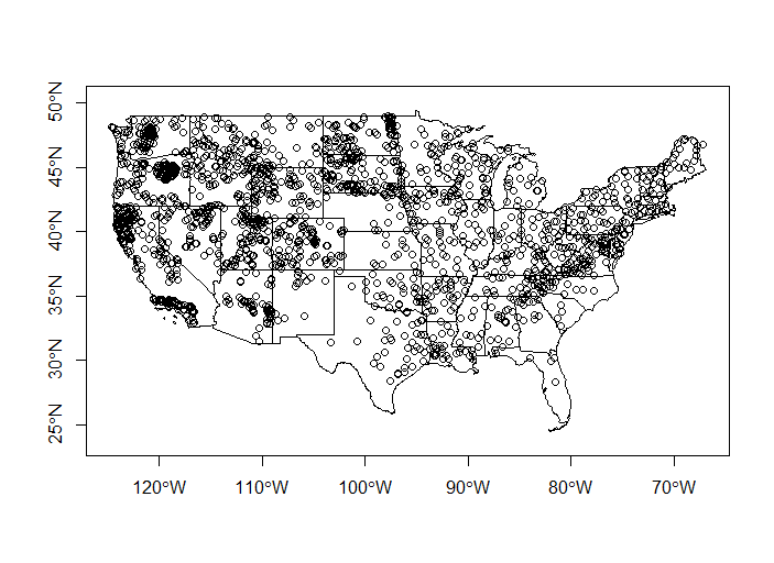
Let’s join the chemistry data to WSA sites - we’re going to summarize the data by states, so let’s also plot all the WSA sites with states to look at
wsa = st_as_sf(wsa, coords = c("LON_DD", "LAT_DD"), crs = 4269,agr = "constant")
states <- st_transform(states, st_crs(wsa))
plot(states$geometry, axes=TRUE)
plot(wsa$geometry, add=TRUE)
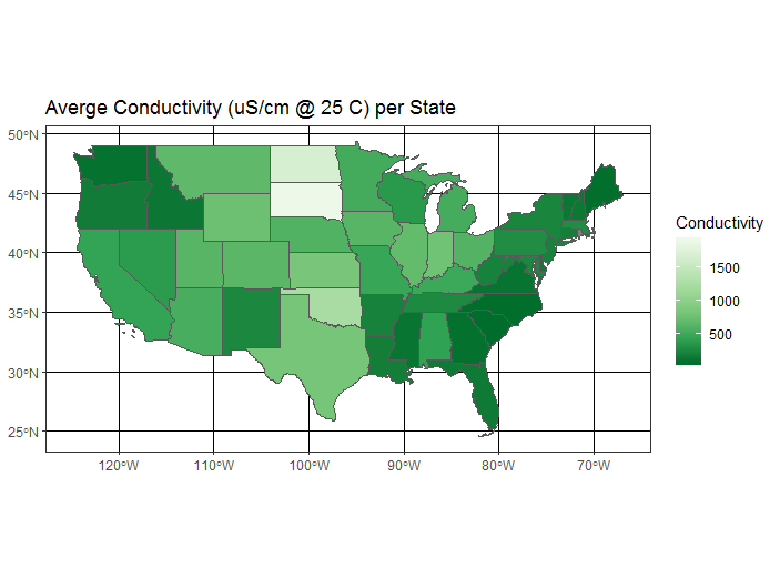
Now we’ll roll together join and dplyr group-by and summarize to get a conducivity per state object which we’ll map using ggplot and geom_sf
avg_cond_state <- st_join(states, wsa) %>%
  dplyr::group_by(name) %>%
  dplyr::summarize(MeanCond = mean(COND, na.rm = TRUE))

ggplot(avg_cond_state) +
  geom_sf(aes(fill = MeanCond)) +
  scale_fill_distiller("Conductivity", palette = "Greens") +
  ggtitle("Averge Conductivity (uS/cm @ 25 C) per State") +
  theme_bw()
Your turn - try summarizing some other data and do perhaps a different summarization method, or change palette in ggplot, etc.
Reading in Spatial Data with sf
We showed earlier how to read in both shapefiles and geodatabase features using sp - let’s do the same with sf. To see what vector data formats you can read / write with sf, type:
st_drivers()
Again, lots and lots of options! Here are a couple quick examples for both shapefile and geodatabase features using st_read in sf (replace my example file paths with file paths to use to working directory on your computer:
Reading in shapefiles:
download.file("http://www.naturalearthdata.com/http//www.naturalearthdata.com/download/110m/cultural/ne_110m_admin_0_countries.zip", "ne_110m_admin_0_countries.zip")
unzip("ne_110m_admin_0_countries.zip", exdir = ".")
countries <- st_read("ne_110m_admin_0_countries.shp")
plot(countries$geometry) # plot it!
Reading in geodatabases - we’ll just recycle geodatabase we use in the sp session:
# Geodatabase Example - if you haven't already downloaded:
download.file("https://www.blm.gov/or/gis/files/web_corp/state_county_boundary.zip","/home/marc/state_county_boundary.zip")
unzip("state_county_boundary.zip", exdir = "/home/marc")
fgdb = "state_county_boundary.gdb"

# List all feature classes in a file geodatabase
st_layers(fgdb)
  layer_name     geometry_type features fields
1 state_poly     Multi Polygon     2825      4
2   cob_poly     Multi Polygon       75      5
3    cob_arc Multi Line String      399      8
# Read the feature class
state_poly = st_read(dsn=fgdb,layer="state_poly")
state_poly$SHAPE