06 - Spatial Data in R - Raster
18 April 2017
While there is an sp SpatialGridDataFrame object to work with rasters in R, the prefered method far and away is to use the newer raster package by Robert J. Hijmans. The raster package has made working with raster data (as well as vector spatial data for some things) much easier and more efficient. The raster package allows you to:
- read and write almost any commonly used raster data format using rgdal
- create rasters, do typical raster processing operations such as resampling, projecting, filtering, raster math, etc.
- work with files on disk that are too big to read into memory in R
- run operations quite quickly since the package relies on back-end C code
The home page for the raster package has links to several well-written vignettes and documentation for the package.
The raster package uses three classes / types of objects to represent raster data - RasterLayer, RasterStack, and RasterBrick - these are all S4 new style classes in R, just like sp classes.
Lesson Goals
- Understand how to create, load, and analyze raster data in R
- Understand basic structure of rasters in R and how to manipulate
- Try some typical GIS-y operations on raster data in R like performing zonal statistics
Quick Links to Exercises
- Exercise 1: Exploratory analysis on raster data
- Exercise 2: Explore Landsat data
- Exercise 3: Zonal Statistics
Let’s create an empty RasterLayer object-
library(raster)
r <- raster(ncol=10, nrow = 10, xmx=-116,xmn=-126,ymn=42,ymx=46)
str(r)
r
r[] <- runif(n=ncell(r))
r
plot(r)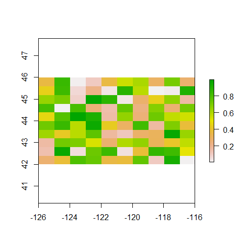
When you look at summary information for the RasterLayer, by simply typing “r”, you’ll notice the main information defining a RasterLayer object described. Minimal information needed to define a RasterLayer include the number of columns and rows, the bounding box or spatial extent of the raster, and the coordinate reference system. What do you notice about the coordinate reference system of raster we just generated from scratch?
You can access raster values via direct indexing or line, column indexing - take a minute to see how this works using raster r we just created - syntax is:
r[i]
r[line, column]
A RasterStack is a raster object with multiple raster layers - essentially a multi-band raster. RasterStack and RasterBrick are very similar and we won’t delve into differences much here - basically, a RasterStack can virtually connect several RasterLayer objects in memory and allows pixel-based calculations on separate raster layers, while a RasterBrick has to refer to a single multi-layer file or multi-layer object. Note that methods that operate on either a RasterStack or RasterBrick usually return a RasterBrick, and processing will be mor efficient on a RasterBrick object.
It’s easy to manipulate our RasterLayer to make a couple new layers, and then stack layers:
r2 <- r * 50
r3 <- sqrt(r * 5)
s <- stack(r, r2, r3)
s
plot(s)
Same process for generating a raster brick (here I make layers and stack, or brick, in same step):
b <- brick(x=c(r, r * 50, sqrt(r * 5)))
b
plot(b)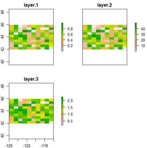
Exercise 1
Exploratory analysis on raster data
Let’s play with some real datasets and perform some simple analyses on some raster data. First let’s grab some boundary spatial polygon data to use in conjuntion with raster data - we’ll grab PNW states using the very handy getData function in raster (you can use help(getData) to learn more about the function). Here we use the global administrative boundaries, or GADM data, to load in US states and subset to the PNW - note how we subset the data and see if you follow how that works.
US <- getData("GADM",country="USA",level=2)
states    <- c('California', 'Nevada', 'Utah','Montana', 'Idaho', 'Oregon', 'Washington')
PNW <- US[US$NAME_1 %in% states,]
plot(PNW, axes=TRUE)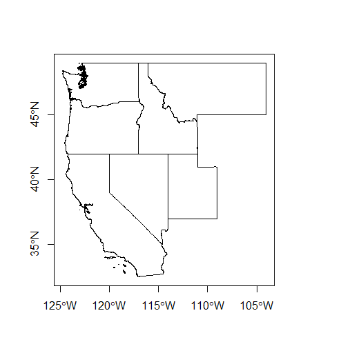
We won’t delve into in this workshop, but if you end up working in R, learn ggplot! For that matter, learn most of Hadley Wickham’s packages which he has rolled into what he now calls tidyverse. Here’s example of plotting same data above using ggplot:
library(ggplot2)
ggplot(PNW) + geom_polygon(data=PNW, aes(x=long,y=lat,group=group),
  fill="cadetblue", color="grey") + coord_equal()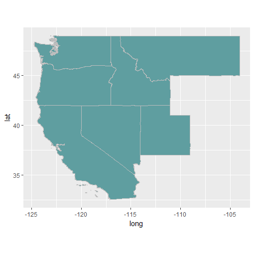
We can also load some raster data using getData - with getData, you can load the following data directly into R to work with:
- SRTM 90 (elevation data with 90m resolution between latitude -60 and 60)
- World Climate Data (Tmin, Tmax, Precip, BioClim)
- Global adm. boundaries (different levels)
Let’s first load some elevation data from SRTM - we need to pass lat and lon, we’ll base roughly on PNW states we just defined:
srtm <- getData('SRTM', lon=-116, lat=42)
plot(srtm)
plot(PNW, add=TRUE)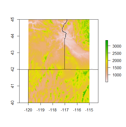
Note that R only allows us to plot our states and SRTM together because they are in the same CRS - typically, in R, we always need to check the CRS of any spatial dataset and project one dataset to CRS of another to plot together or analyze together.
We can see that the tile we pulled only covers a small portion of PNW - let’s pull in a few more tiles, and restrict ourselves to just Oregon so we don’t have to pull too many tiles. I’ll leave it up to you to figure out how to create a new OR SpatialPolygonsDataFrame using same method we used to construct PNW from US.
OR <- PNW[PNW$NAME_1 == 'Oregon',]
srtm2 <- getData('SRTM', lon=-121, lat=42)
srtm3 <- getData('SRTM', lon=-116, lat=47)
srtm4 <- getData('SRTM', lon=-121, lat=47)

srtm_all <- mosaic(srtm, srtm2, srtm3, srtm4,fun=mean)

plot(srtm_all)
plot(OR, add=TRUE)
We have full coverage now for Oregon - we can use crop in raster to crop the SRTM down to the bbox of our OR SpatialPolygonsDataFrame:
srtm_crop_OR <- crop(srtm_all, OR)
plot(srtm_crop_OR, main="Elevation (m) in Oregon")
plot(OR, add=TRUE)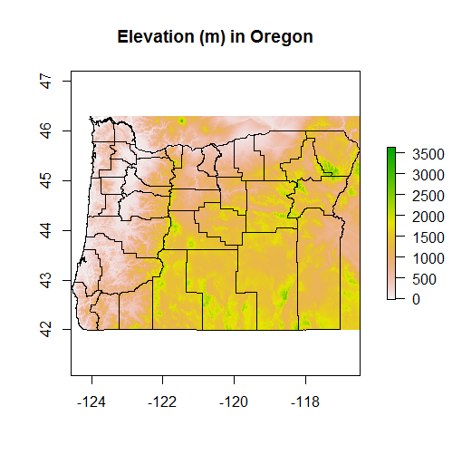
If we wanted to clip to exact boundary of Oregon we would follow crop with mask, but don’t run this, takes too long for entire state of Oregon.
srtm_mask_OR <- crop(srtm_crop_OR, OR)You can verify this by grabbing just a county, and cropping and masking SRTM data with that county:
Benton <- OR[OR$NAME_2=='Benton',]
srtm_crop_Benton <- crop(srtm_crop_OR, Benton)
srtm_mask_Benton <- mask(srtm_crop_Benton, Benton)
plot(srtm_mask_Benton, main="Elevation (m) in Benton County")
plot(Benton, add=TRUE)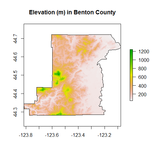
We can play with a number of summary functions for rasters, but perhaps not quite intuitively, these functions (min,max,mean,prod,sum,Median,cv,range,any,all) applied directly to a RasterLayer will return another RasterLayer.
If we want numbers, we’d instead use cellStats. Glance at the help for cellStats if you need to find the syntax and find the mean, min, max, median and range of elevation in Oregon. You’ll have to run the following first - raster values are integers and cellStats balks at this - convert to numeric:
typeof(values(srtm_crop_OR))
values(srtm_crop_OR) <- as.numeric(values(srtm_crop_OR))
typeof(values(srtm_crop_OR))
Try converting values in srtm_crop_OR to feet and then get summary numbers, see if they make sense.
We can do some really cool stuff with the rasterVis package:
library(rasterVis)
histogram(srtm_crop_OR, main="Elevation In Oregon")
densityplot(srtm_crop_OR, main="Elevation In Oregon")
p <- levelplot(srtm_crop_OR, layers=1, margin = list(FUN = median))
p + layer(sp.lines(OR, lwd=0.8, col='darkgray'))
It’s trivial to generate terrain rasters from elevation using raster:
Benton_terrain <- terrain(srtm_mask_Benton, opt = c("slope","aspect",
"tpi","roughness","flowdir"))
plot(Benton_terrain)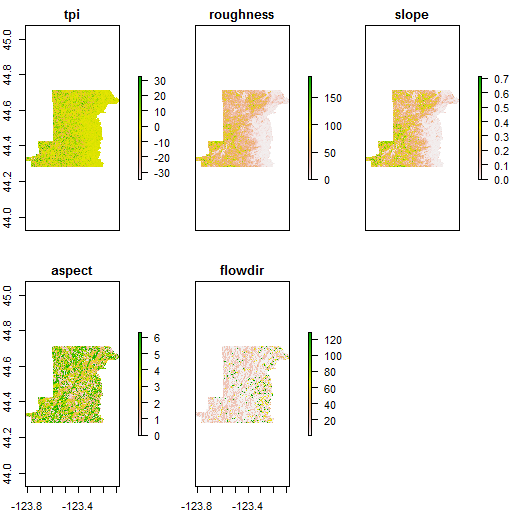
Benton_hillshade <- hillShade(Benton_terrain[['slope']],Benton_terrain[['aspect']])
plot(Benton_hillshade, main="Hillshade Map for Benton County")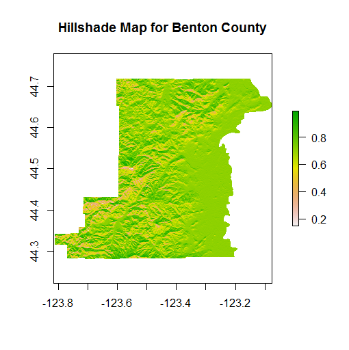
Try making contours of the srtm data for Benton county.
Exercise 2
Explore Landsat data
Let’s try and calulate some different indices with Landsat 7 data usine Sarah Goslee’s handy landsat package. There are a couple sample scenes in the landsat package - each band is loaded as a separate SpatialGridDataFrame. We’ll read in each band of the July scene, convert to raster, and then make a RasterStack. Note that there is also another great package for acquiring Landscat imagery, getlandsat, from ropenscilabs to get Landsat 8 imagery from AWS
library(landsat)
data(july1,july2,july3,july4,july5,july61,july62,july7)
july1 <- raster(july1)
july2 <- raster(july2)
july3 <- raster(july3)
july4 <- raster(july4)
july5 <- raster(july5)
july61 <- raster(july61)
july62 <- raster(july62)
july7 <- raster(july7)
july <- stack(july1,july2,july3,july4,july5,july61,july62,july7)
july
plot(july)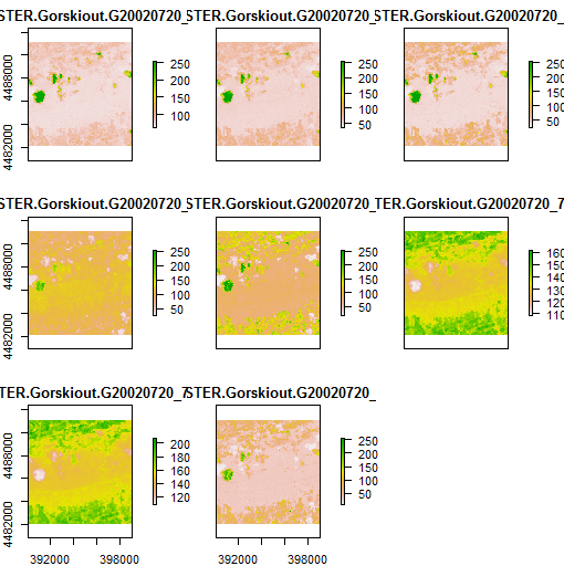
Your task: using the USGS Landsat Product Guide to get specifics of the following Landsat indices, create new RasterLayers of
- Normalized Difference Vegetation Index (NDVI)
- Soil Adjusted Vegetation Index (SAVI)
- Normalized Difference Moisture Index (NDMI)
Remember, this is just simple raster math using the RasterStack bands. Extra credit if you make functions out each process. Remember, if you need help you can look at the source code, but try solving on your own first.
Exercise 3
Zonal Statistics
For this exercise, we’ll use both the SRTM data from earlier and we’ll grab some NLCD data for Oregon from the Oregon Spatial Data Library (I’ve subset the full state NLCD and posted as a zip file on class files folder):
First, let’s try calculating some zonal statistics using a couple Oregon counties as our ‘zones’ and our SRTM data from before as our value raster.
Try working through this one on your own - the solution is posted in the source code if you need help. The steps you’ll need to follow are:
- Create a new
SpatialPolygonsDataFramefrom our earlier ORSpatialPolygonsDataFrameby subsetting like so:
ThreeCounties <- OR[OR$NAME_2 %in% c('Washington','Multnomah','Hood River'),]-
Crop the earlier srtm_crop_OR
RasterLayerusing the new ThreeCountiesSpatialPolygonsDataFrame -
Use
extractin therasterpackage to generate a mean value for each of the three counties.- Hint: Read thoroughly the help for
extract. You will want to use parameter for fun (for mean), na.rm, small, and df. - Extra: Match the county names back to the resulting data frame of mean elevations.
matchis a super handy function in R.
- Hint: Read thoroughly the help for
Next, let’s try to tabulate NLCD land cover for the same three counties. We’ll use a version of NLCD 2011 I grabbed from the Oregon Spatial Data Library and cropped down to our three counties (otherwise too big to work with for class).
download.file("https://github.com/mhweber/gis_in_action_r_spatial/blob/gh-pages/files/NLCD2011.Rdata?raw=true",
              "NLCD2011.Rdata",
              method="auto",
              mode="wb")
Tabulating land use in a raster by spatial polygon regions is a bit trickier than a straight zonal statistics operation in R - some of this may seem a bit confusing, but try and take your time and work through the process. Ideas for tabulating lands use from here and here. Again, try looking through these examples, ask questions, try writing your own approach to solve this based on these examples, but you’ll likely want to work through the source code and see if you can follow how it’s working.
Note that you’re also going to have to reconcile the projections - R won’t allow you to analyze spatial objects in different projections. Hint: you’ll use projection for the RasterLayer and proj4string for the three counties SpatialPolygonsDataFrame - it’s quickest to use spTransform on the three counties and project into same Lambers projection as the NLCD RasterLayer.
What you end up should be a summary of percent of each land use for each of our 3 counties in a nice data frame format.
-
R
rasterResources:OR you can install this as a package and run examples yourself in R: