05 - Spatial Data in R - simple features
18 April 2017
The sf Simple Features for R package by Edzer Pebesma is a new, very nice package that represents a changes of gears from the sp S4 or new style class representation of spatial data in R, and instead provides simple features access for R. This will be familiar to folks who use PostGIS, MySQL Spatial Extensions, Oracle Spatial, the OGR component of the GDAL library, GeoJSON and GeoPandas in Python. Simple features are represented with Well-Known text - WKT - and well-know binary formats.
The big difference is the use of S3 classes in R rather than the S4, or new style classes of sp with the use of slots. Simple features are simply data.frame objects that have a geometry list-column. sf interfaces with GEOS for topolgoical operations, uses GDAL for data creation as well as very speedy I/O along with GEOS, and also which is quite nice can directly read and write to spatial databases such as PostGIS.
Edzar Pebesma has extensive documentation, blog posts and vignettes available for sf here:
Simple Features for R
Lesson Goals
- Learn about new simple features package
First, if not already installed, install sf
library(devtools)
# install_github("edzer/sfr")
library(sf)
## Linking to GEOS 3.5.0, GDAL 2.1.1, proj.4 4.9.3
The sf package has numerous topological methods for performing spatial operations.
methods(class = "sf")
##  [1] [                 aggregate         cbind
##  [4] coerce            initialize        plot
##  [7] print             rbind             show
## [10] slotsFromS3       st_agr            st_agr<-
## [13] st_as_sf          st_bbox           st_boundary
## [16] st_buffer         st_cast           st_centroid
## [19] st_convex_hull    st_crs            st_crs<-
## [22] st_difference     st_drop_zm        st_geometry
## [25] st_geometry<-     st_intersection   st_is
## [28] st_linemerge      st_polygonize     st_precision
## [31] st_segmentize     st_simplify       st_sym_difference
## [34] st_transform      st_triangulate    st_union
## see '?methods' for accessing help and source code
To begin exploring, let’s read in some spatial data. Download Oregon counties from the Oregon Spatial Data Library and load into simple features object - first we get the url for zip file, download and unzip, and then read into a simple features object in R.
library(sf)
counties_zip <- 'http://oe.oregonexplorer.info/ExternalContent/SpatialDataforDownload/orcnty2015.zip'
download.file(counties_zip, '/home/marc/OR_counties.zip')
unzip('/home/marc/OR_counties.zip')
counties <- st_read('orcntypoly.shp')
## Reading layer `orcntypoly' from data source `J:\GitProjects\R-Spatial-Tutorials\orcntypoly.shp' using driver `ESRI Shapefile'
## Simple feature collection with 36 features and 12 fields
## geometry type:  POLYGON
## dimension:      XY
## bbox:           xmin: -124.7038 ymin: 41.99208 xmax: -116.4632 ymax: 46.29239
## epsg (SRID):    4269
## proj4string:    +proj=longlat +datum=NAD83 +no_defs
class(counties)
## [1] "sf" "data.frame"
attr(counties, "sf_column")
## [1] "geometry"
head(counties)
## Simple feature collection with 6 features and 5 fields
## geometry type:  POLYGON
## dimension:      XY
## bbox:           xmin: -124.7038 ymin: 41.99253 xmax: -119.3594 ymax: 43.61744
## epsg (SRID):    4269
## proj4string:    +proj=longlat +datum=NAD83 +no_defs
##   OBJECTID SHAPE_Leng SHAPE_Area     unitID         instName
## 1        1          0          0 1155133033 Josephine County
## 2        1          0          0 1155129015     Curry County
## 3        1          0          0 1135853029   Jackson County
## 4        1          0          0 1135848011      Coos County
## 5        1          0          0 1155134035   Klamath County
## 6        1          0          0 1135854037      Lake County
##                         geometry
## 1 POLYGON((-123.229619367 42....
## 2 POLYGON((-123.811553228 42....
## 3 POLYGON((-122.282727755 42....
## 4 POLYGON((-123.811553228 42....
## 5 POLYGON((-121.332969065 43....
## 6 POLYGON((-119.896580665 43....
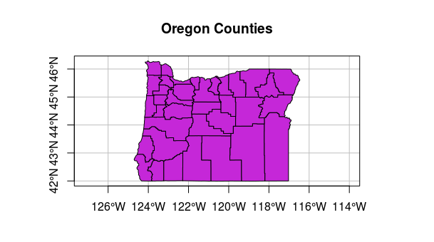
Simple plotting just as with sp spatial objects…note how it’s easy to graticules as a parameter for plot in sf.
plot(counties[1], main='Oregon Counties', graticule = st_crs(counties), axes=TRUE)
Let’s download Oregon cities as well from Oregon Explorer and load into simple features object
cities_zip <- 'http://navigator.state.or.us/sdl/data/shapefile/m2/cities.zip'
download.file(cities_zip, 'C:/users/mweber/temp/OR_cities.zip')
unzip('C:/users/mweber/temp/OR_cities.zip')
cities <- st_read("cities.shp")
## Reading layer `cities' from data source `J:\GitProjects\R-Spatial-Tutorials\cities.shp' using driver `ESRI Shapefile'
## Simple feature collection with 898 features and 6 fields
## geometry type:  POINT
## dimension:      XY
## bbox:           xmin: 238691 ymin: 92141.21 xmax: 2255551 ymax: 1641591
## epsg (SRID):    NA
## proj4string:    +proj=lcc +lat_1=43 +lat_2=45.5 +lat_0=41.75 +lon_0=-120.5 +x_0=399999.9999984001 +y_0=0 +datum=NAD83 +units=ft +no_defs
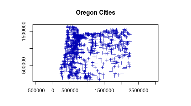
And plotting with plot just like counties - notice use of pch to alter the plot symbols, I personally don’t like the default circles for plotting points in sf.
plot(cities[1], main='Oregon Cities', axes=TRUE, pch=3)
Take a few minutes and try using some simple features functions like st_buffer on the cities or st_centrioid or st_union on the counties and plot to see if it works.
Let’s construct an sf spatial object in R from a data frame with coordinate information - we’ll use the built-in dataset ‘quakes’ with information on earthquakes off the coast of Fiji. Construct spatial points sp, spatial points data frame, and then promote it to a simple features object.
data(quakes)
head(quakes)
##      lat   long depth mag stations
## 1 -20.42 181.62   562 4.8       41
## 2 -20.62 181.03   650 4.2       15
## 3 -26.00 184.10    42 5.4       43
## 4 -17.97 181.66   626 4.1       19
## 5 -20.42 181.96   649 4.0       11
## 6 -19.68 184.31   195 4.0       12
class(quakes)
## [1] "data.frame"
Create a simple features object from quakes
quakes_sf = st_as_sf(quakes, coords = c("long", "lat"), crs = 4326,agr = "constant")
## Classes ‘sf’ and 'data.frame':	1000 obs. of  4 variables:
##  $ depth   : int  562 650 42 626 649 195 82 194 211 622 ...
##  $ mag     : num  4.8 4.2 5.4 4.1 4 4 4.8 4.4 4.7 4.3 ...
##  $ stations: int  41 15 43 19 11 12 43 15 35 19 ...
##  $ geometry:sfc_POINT of length 1000; first list element: Classes 'XY',
## 'POINT', 'sfg'  num [1:2] 181.6 -20.4
## - attr(*, "sf_column")= chr "geometry"
##  ..- attr(*, "names")= chr  "depth" "mag" "stations"
We can use sf methods on quakes now such as st_bbox, st_coordinates, etc.
st_bbox(quakes_sf)
##         min    max
## long 165.67 188.13
## lat  -38.59 -10.72
head(st_coordinates(quakes_sf))
##       X      Y
## 1 181.62 -20.42
## 2 181.03 -20.62
## 3 184.10 -26.00
## 4 181.66 -17.97
## 5 181.96 -20.42
## 6 184.31 -19.68
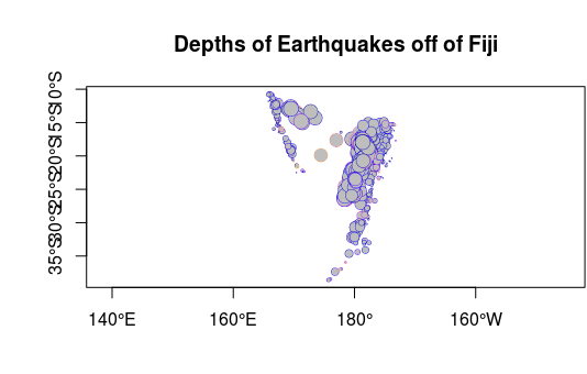
And plot…
plot(quakes_sf[,3],cex=log(quakes_sf$depth/100), pch=21, bg=24, lwd=.4, axes=T)
-
R
sfResources: