Lesson 5 - Exploratory Spatial Data Analysis

22 April 2018

ESDA focuses on visualizing and summarizing both the statistical and spatial distributions of data, with an emphasis on assessing if sites near each other have similar values of an attribute or variable. Detecting such a pattern of spatial autocorrelation could suggest that a spatial data analysis, which uses statistical descriptions and models that incorporate spatial relationships, be used rather than assume observations are indepdent.

Quick Links to Exercises

Exercise 1: ESDA Lagged Scatter Plots: Binning points into Distance Classes
Exercise 2: Points: Creating K-Nearest Neighbor based on Distance
Exercise 3: Polygons: Neighbors based on Contiguity, Moran Scatter Plots and Linked Micromaps

Exercise 1

ESDA Lagged Scatter Plots: Binning points into Distance Classes

One way to conceptualize space for ESDA is by distance. We will use data collected from EPA’s Wadeable Streams Assessment. The Wadeable Streams Assessment is a spatially-balanced, probabilistic survey designed and analyzed using the R package spsurvey. The points, or sites, are from streams sampled in three ecoregions:

Northern Plains
Temperate Plains
Southern Plains.

Olsen et al. (2012) is a good introduction into spatially balanced survey designs, and vignettes on analyzing such surveys are given by Kincaid and Olsen (2016) in the spsurvey package. The lagged scatter plot bins pairs of observations into distance classes. The expectation is the correlation between sites will be highest in the smallest distance class and with increasing distance classes the correlations will be weaker. Dent and Grimm (1999) used lagged scatter plots for ESDA of stream nutrient concentrations.

We’ll use the rgdal package to read ESRI shapelfile with its projection and then take a look at class and summary of the object in R.

library(rgdal)
library(gstat)
library(spdep)

download.file("https://github.com/mhweber/AWRA_GIS_R_Workshop/blob/gh-pages/files/ESDA.zip?raw=true",
              "ESDA.zip",
              method="auto",
              mode="wb")
unzip("ESDA.zip", exdir = ".")
# The shapefile needs to be in the working directory to use '.' or you need to specify the full path in first parameter to readOGR
wsa_plains <- readOGR(".","nplspltpl_bug")

class(wsa_plains)
dim(wsa_plains@data)
names(wsa_plains)
str(wsa_plains, max.level = 2)

## Formal class 'SpatialPointsDataFrame' [package "sp"] with 5 slots
##   ..@ data       :'data.frame':  259 obs. of  285 variables:
##   .. .. [list output truncated]
##   ..@ coords.nrs : num(0) 
##   ..@ coords     : num [1:259, 1:2] 157234 49733 331922 135551 293521 ...
##   .. ..- attr(*, "dimnames")=List of 2
##   ..@ bbox       : num [1:2, 1:2] -1219738 720246 1119139 2928390
##   .. ..- attr(*, "dimnames")=List of 2
##   ..@ proj4string:Formal class 'CRS' [package "sp"] with 1 slot

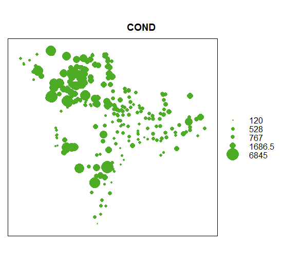
Generate a quick bubble plot

bubble(wsa_plains['COND'])
summary(wsa_plains@data$COND)

BubblePlot

coordinates(wsa_plains)

Generate lagged scatterplots

hscat(COND~1,wsa_plains, c(0, 10000, 50000, 250000, 750000, 1500000, 3000000))

wsa_lagged_scatterplot

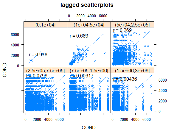
Looking at the smallest distance bin of 0 to 10,000 meters, here is what hscat has plotted. It has calculated all pairwise distances and sorts the data from smallest to largest distance. Beginning with the pair of points with the minimum distance, the conductivity values of that pair are plotted, then the next pair of points having the closest distance are selected and their conductivity values plotted, etc. Here are those first five pairs of points. A log transformation will make seeing those points easier.

FID pairs	Distance (m)	Conductivity (µS/cm)
173:187	6,485	914:1019
212:220	6,577	587:540
107:118	7,545	1071:778
206:236	8,652	732:918
165:179	9,307	3043:2166

The next code chunk continues with lagged scatter plots for log of conductivity.

hscat(log(COND) ~ 1,wsa_plains, c(0, 10000, 50000, 250000, 750000, 1500000, 3000000))
hscat(log(COND) ~ 1,wsa_plains, c(0, 10000, 50000, 100000, 150000, 200000, 250000))
hscat(log(COND) ~ 1,wsa_plains, c(0, 10000, 25000, 50000, 75000, 100000))
hscat(log(PTL) ~ 1,wsa_plains, c(0, 10000, 50000, 250000, 750000, 1500000, 3000000))
hscat(log(PTL) ~ 1,wsa_plains, c(0, 10000, 50000, 100000, 150000, 200000, 250000))
hscat(log(PTL) ~ 1,wsa_plains, c(0, 10000, 25000, 50000, 75000, 100000))

Exercise:

Make lagged scatter plots of total phosphorus concentration, variable PTL. Are those correlations greater or less than the conductivity correlations?
Of the three plains ecoregions, which one has the highest correlation in the first bin of distances for conductivity?

Exercise 2

Points: Creating K-Nearest Neighbor based on Distance

Some spatial data analysis methods require knowing the neighbors in a dataset. Neighbors can be defined by contiguity of polygons, such as for census tracts, counties, or watersheds. Neighbors can also be defined for points, such as by using centroids of counties. We will continue using the WSA points and create their K=1, or first neighbor, by finding the minimum distance at which all sites have a neighbor. Ver Hoef and Temesgen (2013) compare spatial linear models to k-NN methods in mapping and estimating totals from forestry survey data.

tpl <- subset(wsa_plains, ECOWSA9 == "TPL")
coords_tpl <- coordinates(tpl)
tpl_nb <- knn2nb(knearneigh(coords_tpl, k = 1), row.names=tpl$SITE_ID)
tpl_nb1 <- knearneigh(coords_tpl, k = 1)
#using the k=1 object to find the minimum distance at which all sites have a distance-based neighbor
tpl_dist <- unlist(nbdists(tpl_nb,coords_tpl))

##    Min. 1st Qu.  Median    Mean 3rd Qu.    Max. 
##    6485   25900   44630   50350   62560  270500

summary(tpl_dist)#use max distance from summary to assign distance to create neighbors
tplnb_270km <- dnearneigh(coords_tpl, d1=0, d2=271000, row.names=tpl$SITE_ID)
summary(tplnb_270km)

## Neighbour list object:
## Number of regions: 129 
## Number of nonzero links: 2870 
## Percentage nonzero weights: 17.24656 
## Average number of links: 22.24806 
## Link number distribution:
## 
##  1  4  5  6  7  8  9 10 11 12 13 14 15 16 17 18 19 20 21 22 23 25 26 28 29 
##  1  1  1  1  1  6  2  1  3  1  5  3  2 12  6 10  5  2  3  6  2  9  9  5  1 
## 30 31 32 33 34 35 36 37 39 40 41 43 
##  2  1  3  3  4  4  2  3  3  1  3  2 
## 1 least connected region:
## OWW04440-0530 with 1 link
## 2 most connected regions:
## IAW02344-0112 IAW02344-0250 with 43 links

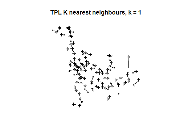
plot(tpl)
plot(knn2nb(tpl_nb1), coords_tpl, add = TRUE)
title(main = "TPL K nearest neighbours, k = 1")

wsa_tpl_knn

Exercise:

What is the distance for knn = 1 for the SPL ecoregion?
The Creating Neighbors vignette from package “spdep” describes other ways to define neighbors. Go to the Packages tab in RStudio, click on spdep, and then click on User guides, package vignettes and other documentation.

Exercise 3

Polygons: Neighbors based on Contiguity, Moran Scatter Plots and Linked Micromaps

In this exercise we are looking at contiguity of catchments and ESDA of land cover of those catchments based on that contiguity. Nelson and Brewer (2015) examined spatial autocorrelation in economic and public health data. In a demonstration we use linked micromaps to summarize both statistical and spatial land cover data at the same time. Finally, we compare the land cover visualization provided by a linked micromap to that of a traditional choropleth map.

library(maptools)
library(rgdal)
library(spdep)
library(stringr)
library(sp)
library(reshape) # for rename function
library(tidyverse)

shp <- readOGR('.', "ef_lmr_huc12")

## OGR data source with driver: ESRI Shapefile 
## Source: "//AA.AD.EPA.GOV/ORD/CIN/USERS/MAIN/L-P/mmcmanus/Net MyDocuments/AWRA GIS 2018/R and Spatial Data Workshop", layer: "ef_lmr_huc12"
## with 815 features
## It has 31 fields

plot(shp)
dim(shp@data)

## [1] 815  31

names(shp@data)

##  [1] "Join_Count" "TARGET_FID" "JOIN_FID"   "GRIDCODE"   "FEATUREID" 
##  [6] "SOURCEFC"   "AreaSqKM"   "OBJECTID"   "HUC_8"      "HUC_10"    
## [11] "HUC_12"     "ACRES"      "NCONTRB_A"  "HU_10_GNIS" "HU_12_GNIS"
## [16] "HU_10_DS"   "HU_10_NAME" "HU_10_MOD"  "HU_10_TYPE" "HU_12_DS"  
## [21] "HU_12_NAME" "HU_12_MOD"  "HU_12_TYPE" "META_ID"    "STATES"    
## [26] "GlobalID"   "SHAPE_Leng" "SHAPE_Area" "GAZ_ID"     "huc12name" 
## [31] "huc12seq"

head(shp@data) # check on row name being used
# Code from Bivand book identifies classes within data frame @ data
# Shows FEATUREID variable as interger
sapply(slot(shp, "data"), class)

## Join_Count TARGET_FID   JOIN_FID   GRIDCODE  FEATUREID   SOURCEFC 
##  "integer"  "integer"  "integer"  "integer"  "integer"   "factor" 
##   AreaSqKM   OBJECTID      HUC_8     HUC_10     HUC_12      ACRES 
##  "numeric"  "integer"   "factor"   "factor"   "factor"  "numeric" 
##  NCONTRB_A HU_10_GNIS HU_12_GNIS   HU_10_DS HU_10_NAME  HU_10_MOD 
##  "numeric"   "factor"   "factor"   "factor"   "factor"   "factor" 
## HU_10_TYPE   HU_12_DS HU_12_NAME  HU_12_MOD HU_12_TYPE    META_ID 
##   "factor"   "factor"   "factor"   "factor"   "factor"   "factor" 
##     STATES   GlobalID SHAPE_Leng SHAPE_Area     GAZ_ID  huc12name 
##   "factor"   "factor"  "numeric"  "numeric"  "integer"   "factor" 
##   huc12seq 
##  "integer"

# Assign row names based on FEATUREID
row.names(shp@data) <- (as.character(shp@data$FEATUREID))
head(shp@data)
tail(shp@data)

# Read in StreamCat data for Ohio River Hydroregion. Check getwd()
scnlcd2011 <- read.csv("NLCD2011_Region05.csv")
names(scnlcd2011)
dim(scnlcd2011)

## [1] 170145     37

class(scnlcd2011)

## [1] "data.frame"

str(scnlcd2011, max.level = 2)
head(scnlcd2011)
scnlcd2011 <- reshape::rename(scnlcd2011, c(COMID = "FEATUREID"))
names(scnlcd2011)

row.names(scnlcd2011) <- scnlcd2011$FEATUREID

head(scnlcd2011)

Example of matching from RWorkflowExampleMWeber.R

# gages$AVE <- gage_flow$AVE[match(gages$SOURCE_FEA,gage_flow$SOURCE_FEA)]
# this matches the FEATUREID from the 815 polygons in shp to the FEATUREID from the df scnlcd2011
efnlcd2011 <- scnlcd2011[match(shp$FEATUREID, scnlcd2011$FEATUREID),]
dim(efnlcd2011)

## [1] 815  37

head(efnlcd2011) # FEATUREID is now row name
row.names(efnlcd2011) <- efnlcd2011$FEATUREID
head(efnlcd2011)
str(efnlcd2011, max.level = 2)
summary(efnlcd2011$PctCrop2011Cat)

##    Min. 1st Qu.  Median    Mean 3rd Qu.    Max. 
##   0.000   4.055  34.580  36.550  66.460 100.000

summary(efnlcd2011$PctDecid2011Cat)

##    Min. 1st Qu.  Median    Mean 3rd Qu.    Max. 
##    0.00   15.84   33.41   36.32   53.79  100.00

Add small constant so log transformation can be done

efnlcd2011 <- efnlcd2011 %>%
    dplyr::mutate(logCrop = log(PctCrop2011Cat + 0.50),
           logDecid = log(PctDecid2011Cat + 0.50))

names(efnlcd2011)

Example code from stackoverflow. Here is how the code works. The match function inside aligns the columns so that order is preserved. So when we merge it with sp@data, order is correctly preserved. A quick check to see if the code has worked is to inspect the two columns corresponding to the common column and see if they are identical (the common columns get duplicated and it is easy to remove the copy, but i keep it as it is a good check) sp@data = data.frame(sp@data, df[match(sp@data[,by], df[,by]),])

shp@data = data.frame(shp@data, efnlcd2011[match(shp@data[,"FEATUREID"], efnlcd2011[,"FEATUREID"]),])

head(shp@data)
class(shp)

## [1] "SpatialPolygonsDataFrame"
## attr(,"package")
## [1] "sp"

names(shp@data)
dim(shp@data)
class(shp@data)
class(shp)
summary(shp)
head(shp@data)
summary(shp@data)

Get centroids of catcments

ctchcoords <- coordinates(shp)
class(ctchcoords)

## [1] "matrix"

Use Rook neighbors

ef.nb1 <- poly2nb(shp, queen = FALSE)
summary(ef.nb1)

## Neighbour list object:
## Number of regions: 815 
## Number of nonzero links: 4632 
## Percentage nonzero weights: 0.6973541 
## Average number of links: 5.683436 
## Link number distribution:
## 
##   1   2   3   4   5   6   7   8   9  10  11  12  13  14  16 
##   3  14  53 170 186 151 115  54  33  19  10   3   2   1   1 
## 3 least connected regions:
## 425 571 666 with 1 link
## 1 most connected region:
## 133 with 16 links

Summary shows there are three catchments with only 1 neighbor and one catchment has 16 neighbors

class(ef.nb1)

## [1] "nb"

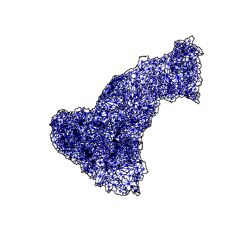
Show neighbors on map of 815 catchments

plot(shp, border = "black")
plot(ef.nb1, ctchcoords, add = TRUE, col = "blue")

eflmr_neighbors

Put Rook neighbors into list

ef.nbwts.list <- nb2listw(ef.nb1, style = "W")
names(ef.nbwts.list)

Moran Scatter Plots:

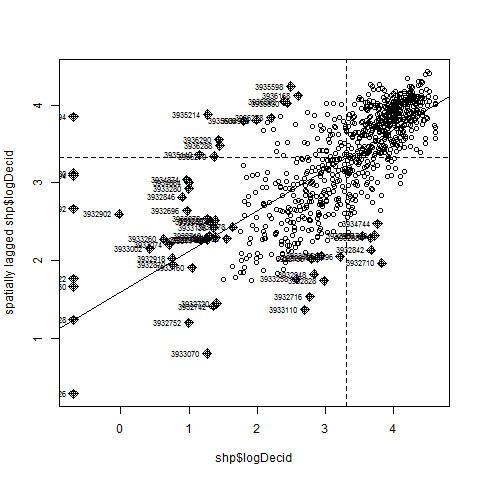
Now that we have neigbors created we can use a Moran scatterplot to compare the percentage of deciduous forest of a focal catchment, which will be plotted on the x-axis, to the average percentage of deciduous forest of its neighboring catchments, with that value plotted on the y-axis. A Moran scatterplot has four quadrats: a high-high in the upper right, a low-low in the lower left, a high-low in the upper left, and a low-high in the lower right. The slope of the line running from the high-high to low-low quadrats is Moran’s I coefficient, measure of spatial autocorrelation. Interactive Moran scatter plots can be made in the GeoDA, which is free and open source spatial data analysis sofware. Spatial data analysis using neighborhood relationships is illustrated in Ver Hoef et al. (2018).

moran.plot(shp$PctDecid2011Cat, listw = ef.nbwts.list, labels = shp$FEATUREID)

eflmr_moranplot

moran.plot(shp$PctDecid2011Cat, listw = ef.nbwts.list, labels = shp$FEATUREID)

Exercise: Make a Moran scatter plot for PctCrop2011Cat. Also, can you write code to make a Moran scatter plot for conductivity based on K = 1 neighbors?

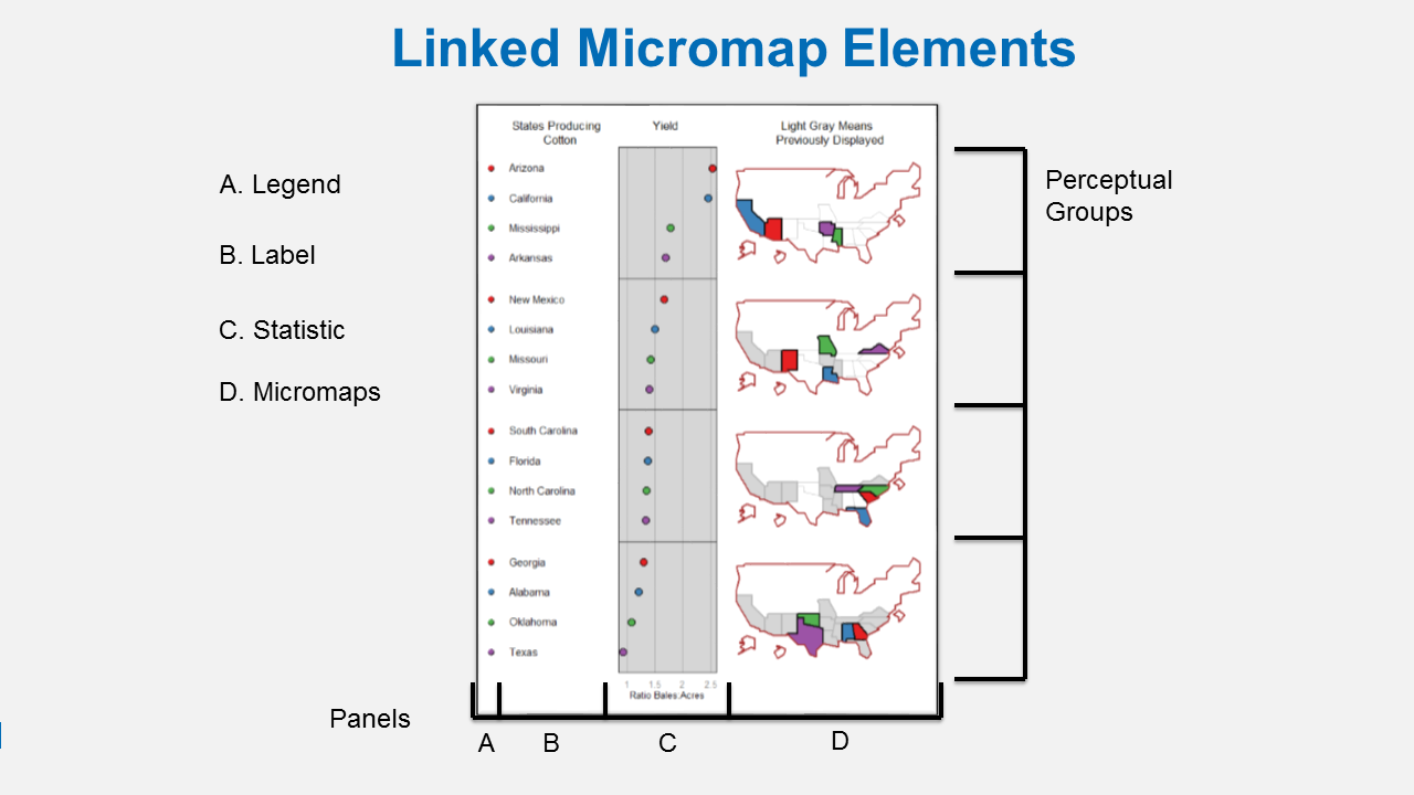
A linked micromap is a graphic that simultaneously summarizes and displays both statistical and geographic distributions by a color-coded link between statistical summaries of polygons to a series of small maps. Here is figure showing the four elements of a linked micromap. Payton et al. (2015) describe the micromap R package.

Linked Micromap Elements

I used linked micromaps to summarize water quality data collected from a spatially, balanced probabilistic stream survey of 25 watersheds done by West Virginia Department of Environmental Protection (McManus et al. 2016). That visualization led to a multivariate spatial analysis based on the contiguity of the watersheds, which was based work done in R by Dray and Jombart (2011) and Dray et al. (2012).

unique(shp@data$huc12name)

##  [1] Moores Fork-SLC          Lucy Run-EFLMR          
##  [3] Backbone Creek-EFLMR     Lick Fork-SLC           
##  [5] Headwaters EFLMR         Salt Run-EFLMR          
##  [7] Todd Run-EFLMR           West Fork EFLMR         
##  [9] Glady Creek-EFLMR        Fivemile Creek-EFLMR    
## [11] Headwaters SLC           Solomon Run-EFLMR       
## [13] Headwaters Dodson Creek  Turtle Creek            
## [15] Anthony Run-Dodson Creek Brushy Fork             
## [17] Cloverlick Creek         Poplar Creek            
## 18 Levels: Anthony Run-Dodson Creek Backbone Creek-EFLMR ... West Fork EFLMR

Create huc12 dataframe for 815 catchment so can slice to get 5 number summary statistics by each huc12

huc12_ds1 <- shp@data
names(huc12_ds1)
str(huc12_ds1) # check huc12names is a factor

From Jeff Hollister EPA NHEERL-AED. The indices [#] pull out the corresponding statistic from the fivenum function

huc12_ds2 <- huc12_ds1 %>%
    group_by(huc12name) %>%
    summarize(decidmin = fivenum(PctDecid2011Cat)[1],
              decidq1 = fivenum(PctDecid2011Cat)[2],
              decidmed = fivenum(PctDecid2011Cat)[3],
              decidq3 = fivenum(PctDecid2011Cat)[4],
              decidmax = fivenum(PctDecid2011Cat)[5],
              cropmin = fivenum(PctCrop2011Cat)[1],
              cropq1 = fivenum(PctCrop2011Cat)[2],
              cropmed = fivenum(PctCrop2011Cat)[3],
              cropq3 = fivenum(PctCrop2011Cat)[4],
              cropmax = fivenum(PctCrop2011Cat)[5])

N.B. using tidyverse function defaults to creating an object that is:

# "tbl_df"     "tbl"        "data.frame"

class(huc12_ds2)

## [1] "tbl_df"     "tbl"        "data.frame"

Huc12_ds2 has the statistical data we want to use - need to specify data.frame in micromap code

devtools::install_github('USEPA/micromap')
library(micromap)

huc12 <- readOGR('.', "ef_lmr_WBD_Sub")
plot(huc12)
names(huc12@data)

huc12.map.table<-create_map_table(huc12,'huc12name')#ID variable is huc12name
head(huc12.map.table)

Draft micromap plot code

mmplot(stat.data = as.data.frame(huc12_ds2),
       map.data = huc12.map.table,
       panel.types = c('dot_legend', 'labels', 'box_summary', 'box_summary', 'map'),
       panel.data=list(NA,
         'huc12name',
         list('cropmin', 'cropq1', 'cropmed', 'cropq3', 'cropmax'),
         list('decidmin', 'decidq1', 'decidmed', 'decidq3', 'decidmax'),
         NA),
       ord.by = 'cropmed',
       rev.ord = TRUE,
       grouping = 6,
       median.row = FALSE,
       map.link = c('huc12name', 'ID'))

Tweaking micromap

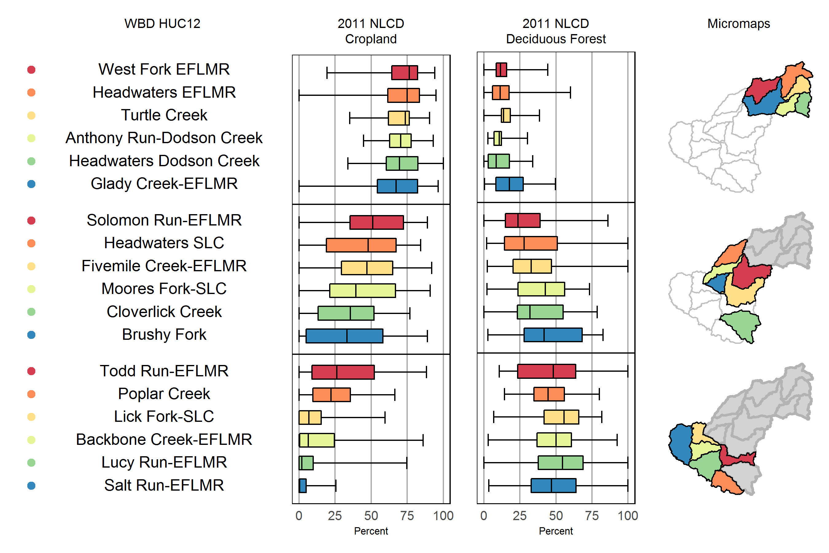
mmplot_lc <- mmplot(stat.data = as.data.frame(huc12_ds2),
       map.data = huc12.map.table,
       panel.types = c('dot_legend', 'labels', 'box_summary', 'box_summary', 'map'),
       panel.data=list(NA,
         'huc12name',
         list('cropmin', 'cropq1', 'cropmed', 'cropq3', 'cropmax'),
         list('decidmin', 'decidq1', 'decidmed', 'decidq3', 'decidmax'),
         NA),
       ord.by = 'cropmed',
       rev.ord = TRUE,
       grouping = 6,
       median.row = FALSE,
       map.link = c('huc12name', 'ID'),
       plot.height=6, plot.width=9,
       colors=brewer.pal(6, "Spectral"),
       
      panel.att=list(list(1, panel.width=.8, point.type=20, point.size=2,point.border=FALSE, xaxis.title.size=1),
                     list(2, header='WBD HUC12', panel.width=1.25, align='center', text.size=1.1),
                     list(3, header='2011 NLCD\nCropland',
graph.bgcolor='white',
xaxis.ticks=c( 0, 25, 50, 75, 100),
xaxis.labels=c(0, 25, 50, 75, 100),
xaxis.labels.size=1,
#xaxis.labels.angle=90,
xaxis.title='Percent',
xaxis.title.size=1,
graph.bar.size = .6),
                     list(4, header='2011 NLCD\nDeciduous Forest',
graph.bgcolor='white',
xaxis.ticks=c( 0, 25, 50, 75, 100),
xaxis.labels=c(0, 25, 50, 75, 100),
xaxis.labels.size=1,
#xaxis.labels.angle=90,
xaxis.title='Percent',
xaxis.title.size=1,
graph.bar.size = .6),
                      list(5, header='Micromaps',
                           inactive.border.color=gray(.7),
                           inactive.border.size=2)))


print(mmplot_lc, name='mmplot_lc_v1_20180205.tiff',res=600)

eflmr_mmplot_lc_v1_20180205

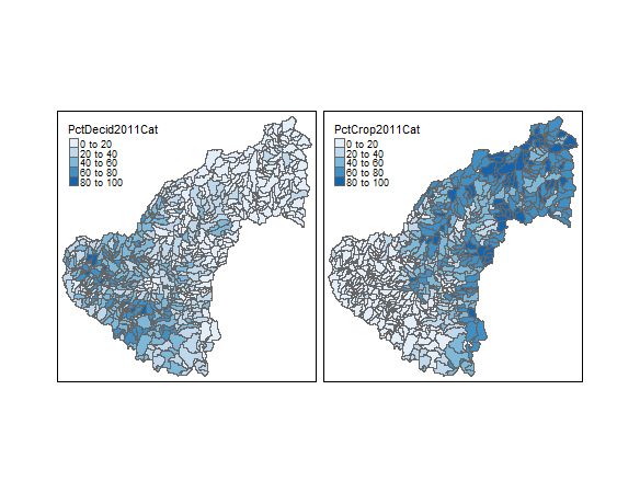
Contrast linked micromap with two choropleth maps

library(tmap)
qtm(shp = shp, fill = c("PctDecid2011Cat", "PctCrop2011Cat"), fill.palette = c("Blues"), ncol =2)

eflmr_choropleth

References

Bivand, R. S., Pebesma, E. J., & Gómez-Rubio, V. (2008). Applied spatial data analysis with R. New York: Springer.
Dent, C. L., and Grimm, N. B. (1999). Spatial heterogeneity of stream water nutrient concentrations over successional time. Ecology, 80(7), 2283-2298.
Dray, S., and Jombart, T. (2011). Revisiting Guerry’s data: Introducing spatial constraints in multivariate analysis. The Annals of Applied Statistics, 5(4), 2278-2299. doi:10.1214/10-AOAS356
Dray, S., Pelissier, R., Couteron, P., Fortin, M. J., Legendre, P., Peres-Neto, P. R., et al. (2012). Community ecology in the age of multivariate multiscale spatial analysis. Ecological Monographs, 82(3), 257-275.
GeoDA
Kincaid, T. M. and Olsen, A. R. (2016). spsurvey: Spatial Survey Design and Analysis. R package version 3.3.
McManus, M. G., Pond, G. J., Reynolds, L., and Griffith, M. B. (2016). Multivariate Condition Assessment of Watersheds with Linked Micromaps. JAWRA Journal of the American Water Resources Association, 52(2), 494-507. doi:10.1111/1752-1688.12399
Nelson, J. K., and Brewer, C. A. (2015). Evaluating data stability in aggregation structures across spatial scales: revisiting the modifiable areal unit problem. Cartography and Geographic Information Science, 1-16.
Olsen, A. R., Kincaid, T. M., and Payton, Q. (2012). Spatially balanced survey designs for natural resources. In R. A. Gitzen, J. J. Millspaugh, A. B. Cooper, and D. S. Licht (Eds.), Design and analysis of long-term ecological monitoring studies (pp. 126-150). Cambridge, UK: Cambridge University Press.
Payton, Q. C., McManus, M. G., Weber, M. H., Olsen, A. R., and Kincaid, T. M. (2015). Micromap: A package for linked micromaps. Journal of Statistical Software, 63(2), 1-16.
Ver Hoef, J. M., Peterson, E. E., Hooten, M. B., Hanks, E. M., and Fortin, M. J. (2018). Spatial autoregressive models for statistical inference from ecological data. Ecological Monographs, 88(1), 36-59.
Ver Hoef, J. M., and Temesgen, H. (2013). A comparison of the spatial linear model to nearest neighbor (k-NN) methods for forestry applications. Plos One, 8(3), e59129.

Lesson 4 - Spatial Data in R - Interactive Mapping Lesson 6 - R ArcGIS Bridge Overview and Demo