Lesson 4 - Spatial Data in R - Interactive Mapping
22 April 2018
There are a number of packages available now in R for mapping and in particular interactive mapping and visualization of spatial data - we’ll take a quick look at a few here. Note that for this section, images on web page here are not interactive (long story….has to do with limitations to the way this GitHub blog site is rendered) - your results, except for using initial ggplot figure, will be interactive.
Lesson Goals
- Explore a sampling of interactive mapping libraries in R
Quick Links to Exercises
- Exercise 1: ggplot and plotly
- Exercise 2: mapview
- Exercise 3: leaflet
- Exercise 4: tmap
- R Mapping Resources
Exercise 1
ggplot and plotly
This first set of examples include gplot and ggmap, which aren’t interactive, but shows using plotly with ggplot map for interactive map
library(ggplot2)
library(plotly)
library(mapview)
library(tmap)
library(leaflet)
library(tidyverse)
library(sf)
library(USAboundaries)
library(ggmap)
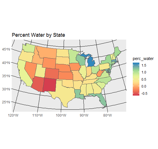
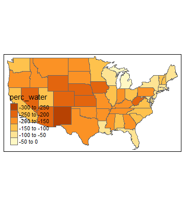
states <- us_states()
states <- states %>%
dplyr::filter(!name %in% c('Alaska','Hawaii', 'Puerto Rico')) %>%
dplyr::mutate(perc_water = log10((awater)/(awater + aland)) *100)
states <- st_transform(states, 5070)
# plot, ggplot
g = ggplot(states) +
geom_sf(aes(fill = perc_water)) +
scale_fill_distiller("perc_water",palette = "Spectral", direction = 1) +
ggtitle("Percent Water by State")
g
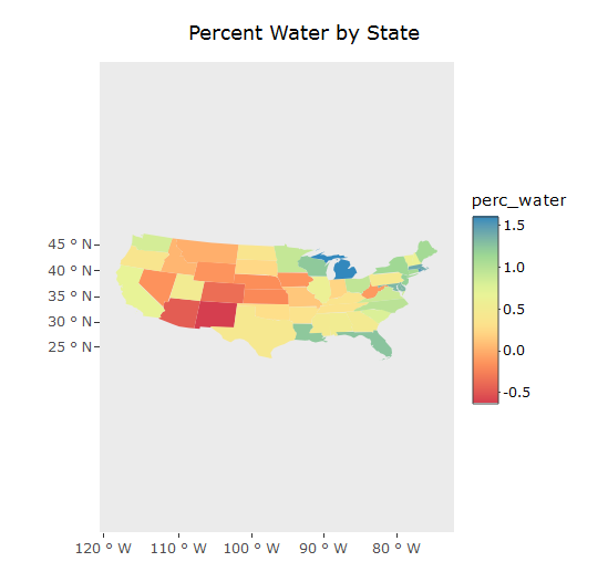
Use plotly to make interactive
ggplotly(g)
Exercise 2
mapview
mapview is a nice package that makes use of leaflet package but simplifies mapping functions. Here again we’ll use the states data pulled in with the USAboundaries package.
mapview(states, zcol = 'perc_water', alpha.regions = 0.2, burst = 'name')
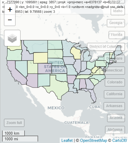
Spend some time playing with parameters in mapview - examine the interactive plot - try different backgrounds, see how you can toggle individual features on and off. mapview can plot rasters as well - try generating a simple map like the one above using one of the raster layers from the raster section. After you plot a raster, see if you can plot multiple layers - mapview makes it easy to plot multiple layers together as described here
Exercise 3
leaflet
Leaflet is an extremely popular open-source javascript library for interactive web mapping, and the leaflet R package allows R users to create Leaflet maps from R. Note that mapview is using Leaflet under the hood and simplifies the mapping process.
The simplest of leaflet maps
m <- leaflet() %>%
addTiles() %>% # Add default OpenStreetMap map tiles
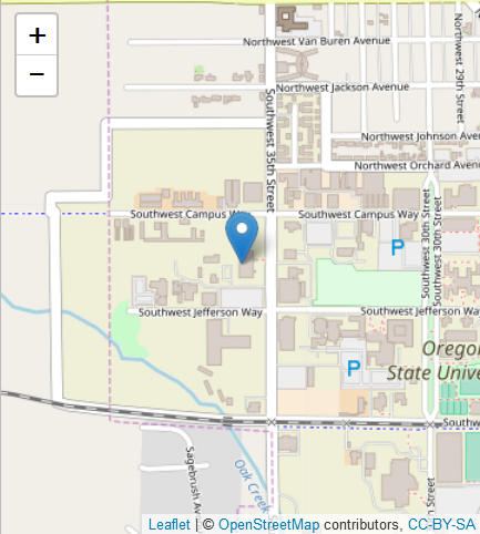
addMarkers(lng=-123.290698, lat=44.565578, popup="Here's where I work")
m # Print the map
Here’s a fun example using geocoding with the ggmap package and looking at where we all came from for this workshop - note that I’m using the the Data Science Toolkit (dsk) API rather than Google Maps API - I found the Google Maps API to be finicky trying to pass city names from multiple states and countries (had to separate out into separate vectors) whereas the dsk API had no trouble at all:
# character vector cities
cities <- c("Stephenville, TX", "Tallahassee, FL" ,"Knoxville, TN","Corvallis, OR","Tampa,FL","Homestead",
            "Fredericksburg, VA","San Diego, CA","Helena, MT","Bedford, NH","Ann Arbor, MI","Morgantown, WV",
            "Raleigh, NC","Boulder, CO","Saint Petersburg, FL", "Beirut, Lebanon", "Kingstown, St Vincent")

places <- geocode(cities, source = "dsk")


locs <- data.frame(cities, places)
str(places)


m <- leaflet(locs) %>%
  addTiles() %>%  # Add default OpenStreetMap map tiles
  addMarkers(lng=locs$lon, lat=locs$lat, popup=locs$cities)
m  # Print the map
# play with provider tiles
m %>% addProviderTiles(providers$Esri.NatGeoWorldMap)
You can add vector (point, line, and polygon) and raster data to leaflet maps. Add our states polygons. Note that you need to set the CRS for states to WGS84 or NAD83 to plot in leaflet as well as transform from sf to sp object - below we do all that in chained dplyr steps.
state_map <- states %>%
  st_transform(crs = 4326) %>%
  as("Spatial") %>%
  leaflet() %>%
  addTiles() %>%
  addPolygons()
Your turn - try adding worldclim raster data using raster getData function to a leaflet map, or try adding one of the raster layers from previous section. Note that with any of the rasters from previous section you’ll need to decrease resolution - see hint here. Try Exploring other provider tiles, but ote that some of the providers do require an API key.
Exercise 4
tmap
tmap is an R package designed for creating thematic maps and based on the layered grammar of graphics approach Hadley Wickham uses with ggplot2. It has a lot of really fantastic functionality - we’ll just touch on very simple examples with datasets we’ve used so far but I’d encourage exploring this package further.
# just fill
tm_shape(states) + tm_fill()
# borders
tm_shape(states) + tm_borders()
# borders and fill
tm_shape(states) + tm_borders() + tm_fill()
tm_shape(states) + tm_borders() + tm_fill(col='perc_water')
You can save a map object and then use layering similar to ggplot2
map_states <- tm_shape(states) + tm_borders()
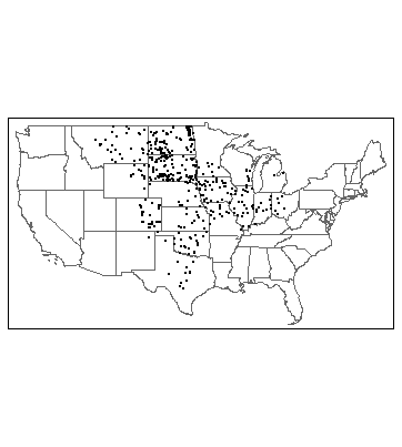
map_states + tm_shape(wsa_plains) + tm_dots()