Testing the rnassqs R package with Willamette basin data

Pull in data via API for Survey data

This script uses the NASS API to query the NASS Quickstats service for historic acres harvested of primary crop groups in Willamette basin counties in Oregon from 1969-2013. An example of using the NASS Quickstats API to pull in and examine crop data in Willamette basin.

library(dplyr)

## Warning: package 'dplyr' was built under R version 3.5.2

library(tibble)
library(tidyr)
library(rnassqs)
library(lubridate)
library(readr)

years <- seq(as.Date('1/1/1969', format="%d/%m/%Y"),as.Date('1/1/2013', format="%d/%m/%Y"),by='years')
years <- sapply(years, function(x) as.numeric(format(x,'%Y')))

i=1
for(y in years){
  # print(y)
  params = list("source_desc"="SURVEY", "sector_desc"="CROPS","year"=y,"state_alpha" = "OR",
              "agg_level_desc"="COUNTY","asd_desc"="NORTHWEST","statisticcat_desc"="AREA HARVESTED")
  d = nassqs(params=params)
  t <- d %>%
    group_by(commodity_desc) %>%
    filter(!county_name %in% c("COLUMBIA","OTHER (COMBINED) COUNTIES")) %>%
    filter(Value != "                 (D)") %>%
    select(year,crop=commodity_desc, Value) %>%
    mutate(Value = as.numeric(gsub("\\,","",Value))) %>%
    summarise(acres_harvested=sum(Value)) %>%
    spread(crop,acres_harvested) 
  
  t <- t %>%
    add_column(Year = y) %>%
    select(Year, everything())
  if (i==1) f <-  t 
  if (i > 1) f <- bind_rows(f,t)
  i=i+1  
}

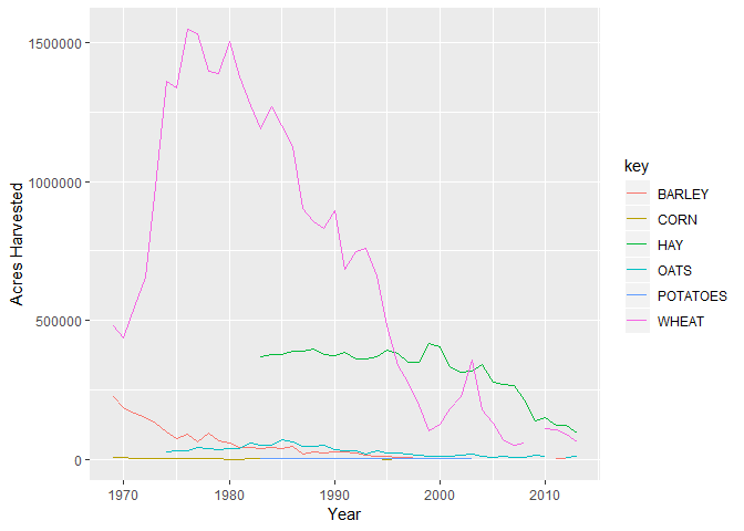
Visualize Survey data

library(ggplot2)
options(scipen=3)
f2 <- gather(f, key, value,-Year)
p1 <- ggplot() + geom_line(aes(y = value, x = Year, colour = key),
                           data = f2, stat="identity") +
  ylab('Acres Harvested')
p1

Compare with NASS Census

This script uses the NASS API to query the NASS Quickstats service for historic acres harvested of primary crop groups in Willamette basin counties in Oregon from 1969 to 2013

years <- c(1997,2002, 2007, 2012, 2017)

i=1
for(y in years){
  # print(y)
  params = list("source_desc"="CENSUS", "sector_desc"="CROPS","year"=y,"state_alpha" = "OR",
                "agg_level_desc"="COUNTY","asd_desc"="NORTHWEST","statisticcat_desc"="AREA HARVESTED")
  d = nassqs(params=params)
  t <- d %>%
    group_by(commodity_desc) %>%
    filter(!county_name %in% c("COLUMBIA","OTHER (COMBINED) COUNTIES")) %>%
    filter(!Value %in% c("                 (D)","                 (Z)")) %>%
    select(year,crop=commodity_desc, Value) %>%
    mutate(Value = as.numeric(gsub("\\,","",Value))) %>%
    dplyr::summarise(acres_harvested=sum(Value)) %>%
    spread(crop,acres_harvested) 
  
  t <- t %>%
    add_column(Year = y) %>%
    select(Year, everything())
  if (i==1) f <-  t 
  if (i > 1) f <- bind_rows(f,t)
  i=i+1  
}

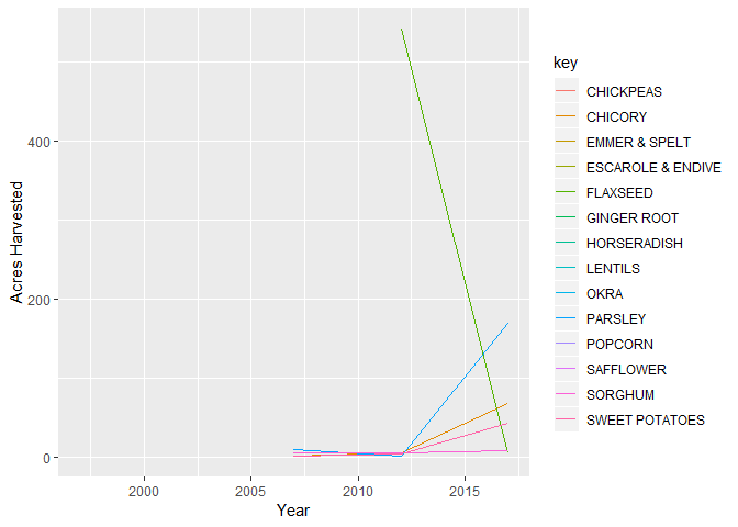
Visualize Census data

f2 <- gather(f[,1:15], key, value,-Year)
p1 <- ggplot() + geom_line(aes(y = value, x = Year, colour = key),
                           data = f2, stat="identity")+
  ylab('Acrea Harvested')
p1

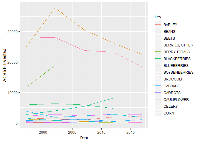
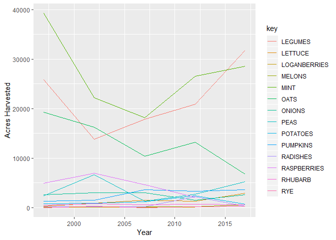
f3 <- gather(f[,c(1,16:29)], key, value,-Year)
p2 <- ggplot() + geom_line(aes(y = value, x = Year, colour = key),
                           data = f3, stat="identity")+
  ylab('Acres Harvested')
p2

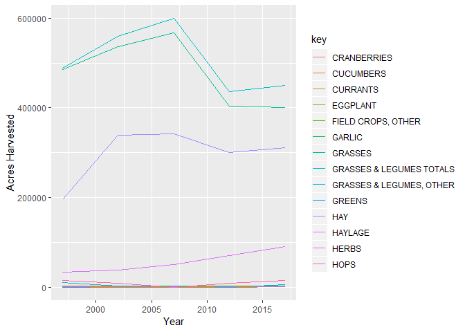
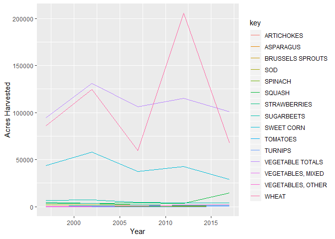
f4 <- gather(f[,c(1,30:43)], key, value,-Year)
p3 <- ggplot() + geom_line(aes(y = value, x = Year, colour = key),
                           data = f4, stat="identity")+
  ylab('Acres Harvested')
p3

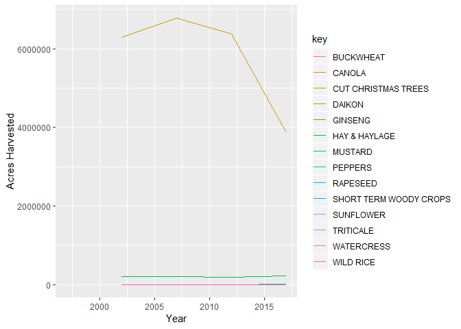
f5 <- gather(f[,c(1,44:58)], key, value,-Year)
p4 <- ggplot() + geom_line(aes(y = value, x = Year, colour = key),
                           data = f5, stat="identity")+
  ylab('Acres Harvested')
p4

f6 <- gather(f[,c(1,59:72)], key, value,-Year)
p5 <- ggplot() + geom_line(aes(y = value, x = Year, colour = key),
                           data = f6, stat="identity")+
  ylab('Acres Harvested')
p5

f7 <- gather(f[,c(1,73:86)], key, value,-Year)
p6 <- ggplot() + geom_line(aes(y = value, x = Year, colour = key),
                           data = f7, stat="identity")+
  ylab('Acres Harvested')
p6