Strava Heatmap

I wanted to create a basic heatmap like you can create based on your activities in Strava. The challenge was downloading / scraping all the data, wrangling it into a format to use, adding an underlying basemap from Stamen and mapping it using ggpmap in R. I bulk downloaded the activies from my Strava account page and then processed in R. I also generated an interactive heatmap with leaflet.

Load Libraries

library(tidyverse)
library(sf)
library(tigris)
library(FITfileR)
library(litedown)
library(R.utils)
library(ggplot2)
library(osmdata)
library(ggmap)
library(leaflet)
library(leaflet.extras)
library(arrow)

Uncompress the downloaded activity data

activities_path <- "C:/Users/mwebe/OneDrive/GitProjects/mhweber.github.io/posts/2025-11-01-Strava-R-map/strava_download/activities"

# gpx_files <- list.files(path = activities_path, pattern = "*.fit.gz", full.names = TRUE)
# 
# 
# # Loop through each .gz file and decompress it
# for (file_path in gpx_files) {
#   base_filename <- basename(file_path)
#   unzipped_filename <- sub("\\.gz$", "", base_filename)
#   gunzip(file_path, remove = FALSE)
# }

fit_files <- list.files(path = activities_path, full.names = TRUE)

Create a function to extract data from all the .fit files

process_fit_files <- function(file_path) {
  if (!file.exists(file_path)) {
    warning(paste("File not found:", file_path))
    return(NULL)
  }

  tryCatch({
    # Read the FIT file
    fit_file <- readFitFile(file_path)

    # Extract 'record' messages, which contain GPS data
    records_list <- records(fit_file)

    if (is.null(records_list) || (is.list(records_list) && length(records_list) == 0)) {
      message(paste("No 'record' messages found in", basename(file_path)))
      return(NULL)
    }

    # Combine potential multiple tibbles (due to different message definitions) into one
    # If it's a single tibble, it's put in a list for consistent processing
    if (is_tibble(records_list)) {
        combined_records <- records_list
    } else {
        combined_records <- bind_rows(records_list)
    }

    # Select key coordinate information and convert to a tibble
    coordinates_data <- combined_records %>%
      select(
        timestamp,
        position_lat,
        position_long,
        # Optional fields, include if they exist
        if ("enhanced_altitude" %in% names(combined_records)) "enhanced_altitude" else if ("altitude" %in% names(combined_records)) "altitude" else NULL,
        if ("distance" %in% names(combined_records)) "distance" else NULL
      ) %>%
      # Remove rows where location data is missing
      na.omit()

    return(coordinates_data)

  }, error = function(e) {
    warning(paste("Error processing file", file_path, ":", e$message))
    return(NULL)
  })
}

Run the function to create a dataframe of all activities

This can take a while if you have many activities

all_data <- map_dfr(fit_files, process_fit_files)

# A tibble: 6 × 6
  timestamp           position_lat position_long altitude distance
  <dttm>                     <dbl>         <dbl>    <dbl>    <dbl>
1 2023-06-21 13:00:16         44.6         -123.     75.6     0.51
2 2023-06-21 13:00:17         44.6         -123.     75.6     1.54
3 2023-06-21 13:00:23         44.6         -123.     75.2     1.54
4 2023-06-21 13:00:25         44.6         -123.     75       6.87
5 2023-06-21 13:00:30         44.6         -123.     74.8    20.0 
6 2023-06-21 13:00:31         44.6         -123.     74.8    22.6 
# ℹ 1 more variable: enhanced_altitude <dbl>

Truncate the data to just local activities within the last year and make spatial

filtered_df <- all_data |> 
  filter(position_lat > 44.5 & position_lat < 44.7) |> 
  filter(position_long > -123.4 & position_long < -123.2) |> 
  filter(timestamp > as.POSIXct("2025-01-01 00:00:00", format = "%Y-%m-%d %H:%M:%S"))
filtered_df_sf <- st_as_sf(filtered_df, coords = c('position_long', 'position_lat'))  |>  st_set_crs(4326)

Bin the data for better viewing in ggmap

binned_data <- filtered_df %>%
  mutate(
    lon_bin = cut(position_long, breaks = 75),
    lat_bin = cut(position_lat, breaks = 75)
  ) %>%
  group_by(lon_bin, lat_bin) %>%
  summarise(count = n(), .groups = 'drop') %>%
  # Convert bin factors back to numeric midpoints for plotting
  mutate(
    lon_mid = as.numeric(sub(',.*', '', sub('\\(', '', lon_bin))) + (as.numeric(sub('.*,', '', sub('\\]', '', lon_bin))) - as.numeric(sub(',.*', '', sub('\\(', '', lon_bin))))/2,
    lat_mid = as.numeric(sub(',.*', '', sub('\\(', '', lat_bin))) + (as.numeric(sub('.*,', '', sub('\\]', '', lat_bin))) - as.numeric(sub(',.*', '', sub('\\(', '', lat_bin))))/2
  )

binned_data_sf <- st_as_sf(binned_data, coords = c('lon_mid', 'lat_mid'))  |>  st_set_crs(4326)

Get Stamen background map

# Get the map tiles
map_bbox <-c(left = -123.4, bottom = 44.5, right = -123.2, top = 44.7)
base_map <- get_stadiamap(bbox = map_bbox, zoom = 12, maptype = "stamen_terrain_lines")

Get background roads as an sf object

First query for hiking trails within the bounding box of activity data. Then convert the osm data to an sf object and extract just the trail line features

roads <- roads("OR", c("Benton","Polk"), progress_bar = FALSE)
roads <- roads |> 
  st_transform(roads,crs=st_crs(filtered_df_sf)) |> 
  st_crop(st_bbox(filtered_df_sf))

Warning: attribute variables are assumed to be spatially constant throughout
all geometries

Make a static map with ggmap

ggmap(base_map) +
  geom_tile(data=binned_data, aes(x = lon_mid, y = lat_mid, fill = count)) +
  scale_fill_gradientn(colors = c("blue", "green", "yellow", "red")) + # Customize color scale
  theme_minimal() +
  labs(title = "Strava Activity Density Heatmap", fill = "Activity Count") +
  coord_fixed(ratio = 1.3)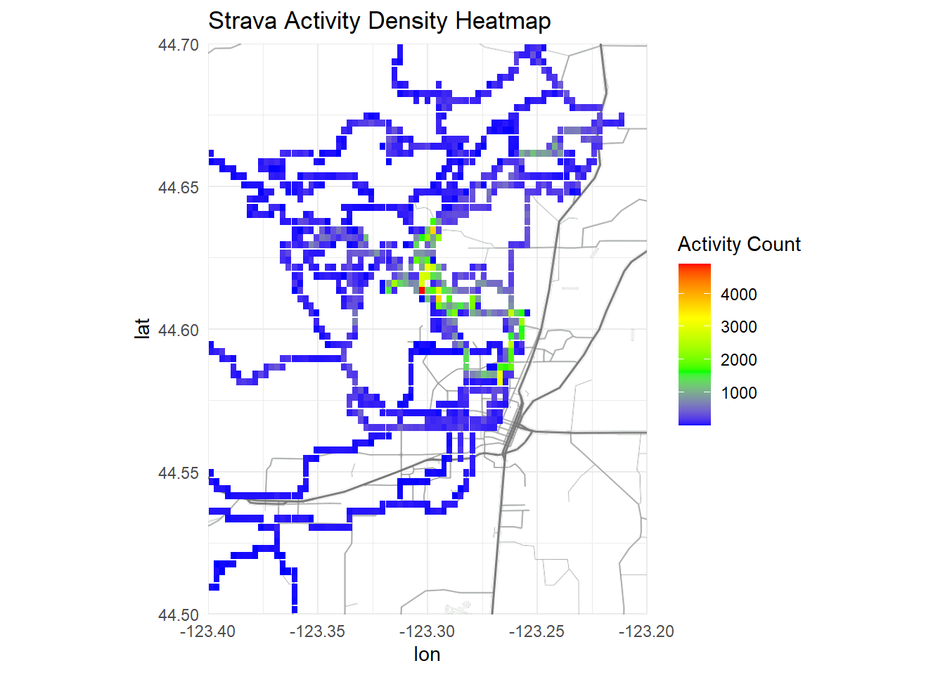

A more pleasing static map with ggplot and cowplot

Inspired by great example of mapping Strava data in this great R-bloggers post

p <- ggplot() + 
  # Construct the Heatmap Portion
  stat_density2d(data = filtered_df,
                 aes(x = position_long, y = position_lat, fill = after_stat(count)),
                 geom = 'tile',
                 contour = F,
                 n = 1000
                 ) +
  #Draw the map local trails
  geom_sf(data = roads, color = '#DDDDDD', alpha = .15) + 
  scale_fill_viridis_c(option = "B", guide = F) +
  ggthemes::theme_map() + 
  theme(
    panel.background = element_rect(fill = 'black'),
    plot.background = element_rect(fill = 'black')
  )

cowplot::ggdraw(p) + 
  labs(title = "My Trails Heatmap",
       caption = "An Adventure with scraping Strava data and mapping in R") +
  theme(panel.background = element_rect(fill = "black"),
        plot.background = element_rect(fill = 'black'),
        plot.title = element_text(color = "#DDDDDD",
                                  family = 'Calibri',
                                  #face = 'bold',
                                  size = 18),
        plot.caption = ggtext::element_markdown(color = '#DDDDDD',
                                    family = 'Calibri',
                                    size = 12))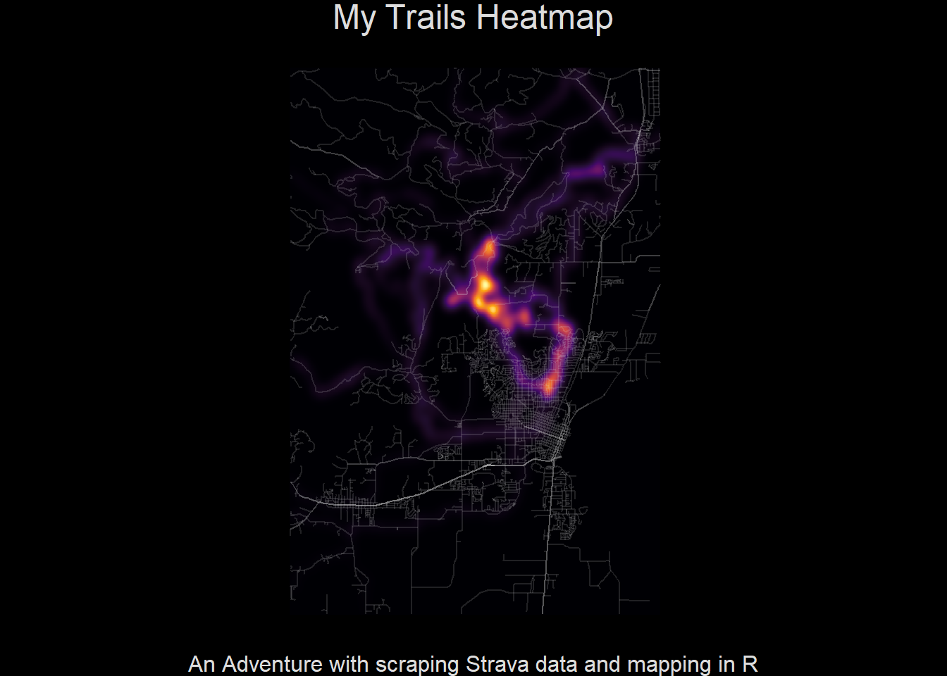

Make an interactive heatmap with leaflet

Also, just for fun, make a simple interactive leaflet map

run_map <- filtered_df  |> 
  leaflet()  |> 
  addTiles()  |>  # Add default OpenStreetMap map tiles
  addHeatmap(
    lng = ~position_long,
    lat = ~position_lat,
    blur = 20,    # Adjust blur and radius for desired look
    max = 0.5,
    radius = 15,
  )

# Display the map
run_map