This is an implementation of the excellent PostGIS / geopandas tutorial here using NHDPlus WBD polygons for PNW. All the ideas and methods are from this tutorial, simply implementing with a different dataset and in Oregon.
%matplotlib inline

import os
import json
import psycopg2

import matplotlib.pyplot as plt
# The two statemens below are used mainly to set up a plotting
# default style that's better than the default from matplotlib
import seaborn as sns
plt.style.use('bmh')

from shapely.geometry import Point
import pandas as pd
import geopandas as gpd
from geopandas import GeoSeries, GeoDataFrame
Connect to PostGIS database of NHDPlus, select WBD features that are in Oregon, and load into a geopandas geodataframe.
con = psycopg2.connect(database="nhdplus", user="postgres",password="postgres",host="localhost",port="5432")
sql= "SELECT * FROM wbd_subwatershed WHERE states = 'OR'"
wbd=gpd.GeoDataFrame.from_postgis(sql, con, geom_col='geom',crs={'init': u'epsg:4326'})
con.close()
len(wbd)
3875
Check out first feature using .iloc (could use wbd.head() also)
wbd.iloc[0]
gid                                                         793
objectid                                                  95489
huc_8                                                  17100306
huc_10                                               1710030604
huc_12                                             171003060402
acres                                                  0.246648
ncontrb_a                                                     0
hu_10_gnis                                                 None
hu_12_gnis                                                 None
hu_10_name                   Euchre Creek-Frontal Pacific Ocean
hu_10_mod                                                    NM
hu_10_type                                                    F
hu_12_ds                                           171003060500
hu_12_name                   Mussel Creek-Frontal Pacific Ocean
hu_12_mod                                                    NM
hu_12_type                                                    I
meta_id                                                    OR04
states                                                       OR
globalid                 {E9EA2E61-1E74-41BB-AC4B-F1568B110DF9}
shape_leng                                            0.0013213
shape_area                                          1.09467e-07
gaz_id                                                   -71052
geom          (POLYGON ((-124.3979671835871 42.5876281986771...
Name: 0, dtype: object
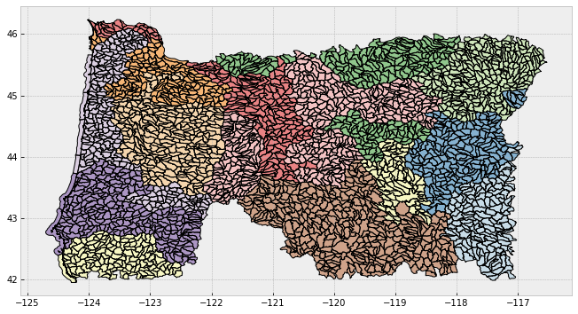
Make a map of WBD polygons and color by 8-digit HUC number
wbd.plot(column='huc_8', cmap='Paired', categorical=True, figsize=(14,6))
<matplotlib.axes._subplots.AxesSubplot at 0x1fe76d30>
Now try dissolving WBD HUC12 polygons using the HUC_8 field to make new HUC8 geodataframe. We’ll keep all the HUC ID and name fields in resulting dissolved geodataframe.
type(wbd)
geopandas.geodataframe.GeoDataFrame
huc8 = wbd.dissolve('huc_8')
len(huc8)
79
Re-apply crs to file (and verify it’s missing first and it’s back after)
print huc8.crs
None
huc8.crs = wbd.crs
print huc8.crs
{'init': u'epsg:4326'}
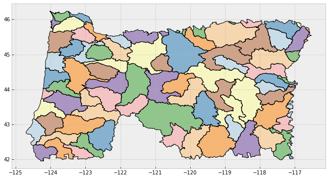
Now plot the dissolved 8-digit HUC polygons-
huc8.plot(cmap = 'Paired', categorical=True, figsize=(14,6));
Project to Oregon statewide Lambert projection - using pyepsg - and then reproject
import pyepsg
pyepsg.get('2991')
<ProjectedCRS: 2991, NAD83 / Oregon LCC (m)>
huc8 = huc8.to_crs(epsg=2991)
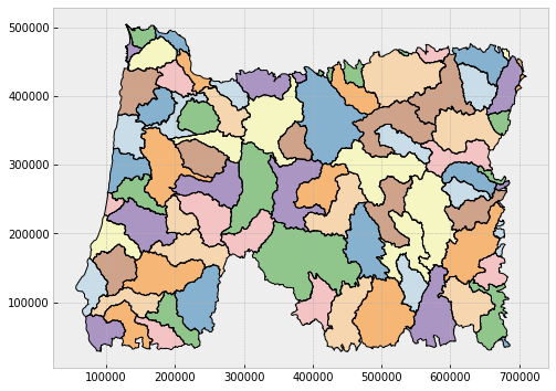
Now plot the re-projected geodataframe
huc8.plot(cmap = 'Paired', categorical=True, figsize=(14,6));
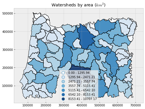
Plot choropleth map using HUC area - and convert area to kilometers (map projection is in meters)
huc8['area_km2'] = huc8.geom.area * 1e-6
huc8.iloc[[0,1,2],[0,22]]
| geom | area_km2 | |
|---|---|---|
| huc_8 | ||
| 17050103 | (POLYGON ((679446.0847084918 184070.6811281344... | 386.085209 |
| 17050106 | POLYGON ((680084.8704586171 49496.81553380163,... | 98.131472 |
| 17050107 | POLYGON ((664255.7335354568 39951.32383508176,... | 2590.766262 |
f, ax = plt.subplots(1, figsize=(8, 6))
huc8.plot(column='area_km2', scheme='fisher_jenks', k=7,
                         alpha=0.9, cmap=plt.cm.Blues, legend=True,ax=ax)
plt.axis('equal')
ax.set_title('Watersheds by area ($km^2$)')
<matplotlib.text.Text at 0x23840a58>
Try a spatial join of polygons on points - I’ll use a set of USGS stream gages I have handy for the point layer.
gages = pd.read_csv('c:/users/mweber/temp/streamgages.csv')
gages.iloc[0]
SOURCE_FEA                          14361500
EVENTTYPE                         StreamGage
STATION_NM    ROGUE RIVER AT GRANTS PASS, OR
STATE                                     OR
LON_SITE                            -123.318
LAT_SITE                             42.4304
Name: 0, dtype: object
Promote the pandas dataframe to a geodataframe using the lattitude and longitude
from shapely.geometry import Point

geometry = [Point(xy) for xy in zip(gages.LON_SITE, gages.LAT_SITE)]
crs = {'init': 'epsg:4326'}
gages = GeoDataFrame(gages, crs=crs, geometry=geometry)
type(gages)
geopandas.geodataframe.GeoDataFrame
gages.iloc[0]
SOURCE_FEA                             14361500
EVENTTYPE                            StreamGage
STATION_NM       ROGUE RIVER AT GRANTS PASS, OR
STATE                                        OR
LON_SITE                               -123.318
LAT_SITE                                42.4304
geometry      POINT (-123.31783647 42.43039607)
Name: 0, dtype: object
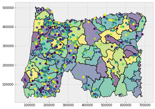
Restrict gages to just Oregon, reproject the gages to the huc8 proojection, then rename the huc8 ‘geom’ column to ‘geometry’ and then we’ll try an inner spatial join
from geopandas.tools import sjoin
#gages = gages.to_crs(epsg=2991)
huc8 = huc8.rename(columns={'geom': 'geometry'}).set_geometry('geometry')
gages.crs == huc8.crs
gages = gages.loc[gages['STATE']=='OR']
gages_huc8 = gpd.sjoin(gages, huc8, how='inner')
f, ax = plt.subplots(1, figsize=(8, 6))
plt.axis('equal')
huc8.plot(ax=ax)
gages_huc8.plot(markersize=6, categorical=True, ax=ax)
<matplotlib.axes._subplots.AxesSubplot at 0x3a84f1d0>
Now run zonal statistics using polygons and rasters with rasterstats
import rasterio
import rasterio.plot as rioplot
import numpy as np
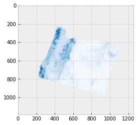
with rasterio.open('H:/WorkingData/Prism_30yr_OR.tif') as src:
transform = src.meta['transform']
precip = src.read(1)
precip[precip < 0] = np.nan
Look at raster metadata
src.meta
{'count': 1,
 'crs': CRS({u'lon_0': -96, u'datum': u'NAD83', u'y_0': 0, u'no_defs': True, u'proj': u'aea', u'x_0': 0, u'units': u'm', u'lat_2': 45.5, u'lat_1': 29.5, u'lat_0': 23}),
 'driver': u'GTiff',
 'dtype': 'float32',
 'height': 1187,
 'nodata': -9999.0,
 'transform': Affine(800.0, 0.0, -2472125.020833,
       0.0, -800.0, 3080024.0625),
 'width': 1259}
rioplot.show(precip, with_bounds=True, cmap=plt.cm.Blues)
<matplotlib.axes._subplots.AxesSubplot at 0x2e9ca860>
import rasterstats as rs
import fiona
#huc8 = huc8.to_crs('+proj=aea +lat_1=29.5 +lat_2=45.5 +lat_0=23 +lon_0=-96 +x_0=0 +y_0=0 +datum=NAD83 +units=m +no_defs +ellps=GRS80 +towgs84=0,0,0')
precip_zonal = rs.zonal_stats(huc8, 'H:/WorkingData/Prism_30yr_OR.tif', geojson_out=True)
precip_zonal = GeoDataFrame.from_features(precip_zonal)
precip_zonal.head(2)
| acres | count | gaz_id | geometry | gid | globalid | hu_10_gnis | hu_10_mod | hu_10_name | hu_10_type | ... | huc_12 | max | mean | meta_id | min | ncontrb_a | objectid | shape_area | shape_leng | states | |
|---|---|---|---|---|---|---|---|---|---|---|---|---|---|---|---|---|---|---|---|---|---|
| 0 | 22381.271444 | 600 | -72812 | (POLYGON ((-1684470.024757544 2449556.42795410... | 2553 | {BC0BA51C-9970-43C3-A810-C6F12B99911A} | None | NM | Lower Succor Creek | S | ... | 170501030901 | 620.897461 | 308.655677 | OR01 | 229.144257 | 0.0 | 103018 | 0.010043 | 0.530808 | OR |
| 1 | 24225.748801 | 154 | -78734 | POLYGON ((-1719043.984217515 2318687.346051499... | 8475 | {BF6E742F-F812-4F50-AF09-B55A52CAE3CC} | None | NM | Tent Creek | S | ... | 170501060502 | 367.764740 | 327.508903 | OR01 | 313.125732 | 0.0 | 220900 | 0.010666 | 0.628540 | OR |
2 rows × 26 columns
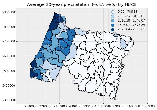
Now a choropleth map of 30-year average precip by 8-digit HUC in Oregon
f, ax = plt.subplots(1, figsize=(8, 6))
precip_zonal.plot(column='mean', scheme='Equal_Interval', k=5,
                   alpha=1, cmap=plt.cm.Blues, legend=True, ax=ax)
plt.axis('equal')
ax.set_title('Average 30-year precipitation ($mm/month$) by HUC8');