Load and look at basics of simple features package
library(devtools)
# install_github("edzer/sfr")
library(sf)
## Linking to GEOS 3.5.0, GDAL 2.1.1, proj.4 4.9.3
nc <- st_read(system.file("shape/nc.shp", package="sf"))
## Reading layer `nc' from data source `C:\Users\mweber\R\library\sf\shape\nc.shp' using driver `ESRI Shapefile'
## converted into: MULTIPOLYGON
## Simple feature collection with 100 features and 14 fields
## geometry type:  MULTIPOLYGON
## dimension:      XY
## bbox:           xmin: -84.32385 ymin: 33.88199 xmax: -75.45698 ymax: 36.58965
## epsg (SRID):    4267
## proj4string:    +proj=longlat +datum=NAD27 +no_defs
class(nc)
## [1] "sf" "data.frame"
attr(nc, "sf_column")
## [1] "geometry"
methods(class = "sf")
##  [1] [                 aggregate         cbind
##  [4] coerce            initialize        plot
##  [7] print             rbind             show
## [10] slotsFromS3       st_agr            st_agr<-
## [13] st_as_sf          st_bbox           st_boundary
## [16] st_buffer         st_cast           st_centroid
## [19] st_convex_hull    st_crs            st_crs<-
## [22] st_difference     st_drop_zm        st_geometry
## [25] st_geometry<-     st_intersection   st_is
## [28] st_linemerge      st_polygonize     st_precision
## [31] st_segmentize     st_simplify       st_sym_difference
## [34] st_transform      st_triangulate    st_union
## see '?methods' for accessing help and source code
head(nc)
## Simple feature collection with 6 features and 14 fields
## geometry type:  MULTIPOLYGON
## dimension:      XY
## bbox:           xmin: -81.74107 ymin: 36.07282 xmax: -75.77316 ymax: 36.58965
## epsg (SRID):    4267
## proj4string:    +proj=longlat +datum=NAD27 +no_defs
##    AREA PERIMETER CNTY_ CNTY_ID        NAME  FIPS FIPSNO CRESS_ID BIR74
## 1 0.114     1.442  1825    1825        Ashe 37009  37009        5  1091
## 2 0.061     1.231  1827    1827   Alleghany 37005  37005        3   487
## 3 0.143     1.630  1828    1828       Surry 37171  37171       86  3188
## 4 0.070     2.968  1831    1831   Currituck 37053  37053       27   508
## 5 0.153     2.206  1832    1832 Northampton 37131  37131       66  1421
## 6 0.097     1.670  1833    1833    Hertford 37091  37091       46  1452
##   SID74 NWBIR74 BIR79 SID79 NWBIR79                       geometry
## 1     1      10  1364     0      19 MULTIPOLYGON(((-81.47275543...
## 2     0      10   542     3      12 MULTIPOLYGON(((-81.23989105...
## 3     5     208  3616     6     260 MULTIPOLYGON(((-80.45634460...
## 4     1     123   830     2     145 MULTIPOLYGON(((-76.00897216...
## 5     9    1066  1606     3    1197 MULTIPOLYGON(((-77.21766662...
## 6     7     954  1838     5    1237 MULTIPOLYGON(((-76.74506378...
Download Oregon counties from Oregon Explorer data and load into simple features object
library(sf)
# Get the url for zip file, download and unzip
# counties_zip <- 'http://oe.oregonexplorer.info/ExternalContent/SpatialDataforDownload/orcnty2015.zip'
# download.file(counties_zip, 'C:/users/mweber/temp/OR_counties.zip')
# unzip('C:/users/mweber/temp/OR_counties.zip')
# Now read into a simple features object in R
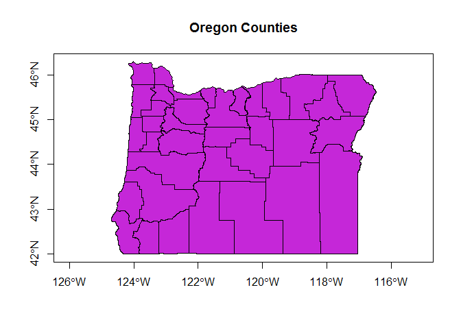
counties <- st_read('orcntypoly.shp')
## Reading layer `orcntypoly' from data source `J:\GitProjects\R-Spatial-Tutorials\orcntypoly.shp' using driver `ESRI Shapefile'
## Simple feature collection with 36 features and 12 fields
## geometry type:  POLYGON
## dimension:      XY
## bbox:           xmin: -124.7038 ymin: 41.99208 xmax: -116.4632 ymax: 46.29239
## epsg (SRID):    4269
## proj4string:    +proj=longlat +datum=NAD83 +no_defs
# simple plot with base R
plot(counties[1], main='Oregon Counties', axes=TRUE)
# the data frame
head(counties[,1:5])
## Simple feature collection with 6 features and 5 fields
## geometry type:  POLYGON
## dimension:      XY
## bbox:           xmin: -124.7038 ymin: 41.99253 xmax: -119.3594 ymax: 43.61744
## epsg (SRID):    4269
## proj4string:    +proj=longlat +datum=NAD83 +no_defs
##   OBJECTID SHAPE_Leng SHAPE_Area     unitID         instName
## 1        1          0          0 1155133033 Josephine County
## 2        1          0          0 1155129015     Curry County
## 3        1          0          0 1135853029   Jackson County
## 4        1          0          0 1135848011      Coos County
## 5        1          0          0 1155134035   Klamath County
## 6        1          0          0 1135854037      Lake County
##                         geometry
## 1 POLYGON((-123.229619367 42....
## 2 POLYGON((-123.811553228 42....
## 3 POLYGON((-122.282727755 42....
## 4 POLYGON((-123.811553228 42....
## 5 POLYGON((-121.332969065 43....
## 6 POLYGON((-119.896580665 43....
Download Oregon cities from Oregon Explorer data and load into simple features object
# cities_zip <- 'http://navigator.state.or.us/sdl/data/shapefile/m2/cities.zip'
# download.file(cities_zip, 'C:/users/mweber/temp/OR_cities.zip')
# unzip('C:/users/mweber/temp/OR_cities.zip')
cities <- st_read("cities.shp")
## Reading layer `cities' from data source `J:\GitProjects\R-Spatial-Tutorials\cities.shp' using driver `ESRI Shapefile'
## Simple feature collection with 898 features and 6 fields
## geometry type:  POINT
## dimension:      XY
## bbox:           xmin: 238691 ymin: 92141.21 xmax: 2255551 ymax: 1641591
## epsg (SRID):    NA
## proj4string:    +proj=lcc +lat_1=43 +lat_2=45.5 +lat_0=41.75 +lon_0=-120.5 +x_0=399999.9999984001 +y_0=0 +datum=NAD83 +units=ft +no_defs
plot(cities[1])

library(sp)
data(quakes)
head(quakes)
##      lat   long depth mag stations
## 1 -20.42 181.62   562 4.8       41
## 2 -20.62 181.03   650 4.2       15
## 3 -26.00 184.10    42 5.4       43
## 4 -17.97 181.66   626 4.1       19
## 5 -20.42 181.96   649 4.0       11
## 6 -19.68 184.31   195 4.0       12
class(quakes)
## [1] "data.frame"
# Data frames consist of rows of observations on columns of values for variables of interest. Create the coordinate reference system to use
llCRS <- CRS("+proj=longlat +datum=NAD83")
# now stitch together the data frame coordinate fields and the
# projection string to createa SpatialPoints object
quakes_sp <- SpatialPoints(quakes[, c('long', 'lat')], proj4string = llCRS)
# Summary method gives a description of the spatial object in R. Summary works on pretty much all objects in R - for spatial data, gives us basic information about the projection, coordinates, and data for an sp object if it's a spatial data frame object.
summary(quakes_sp)
## Object of class SpatialPoints
## Coordinates:
##         min    max
## long 165.67 188.13
## lat  -38.59 -10.72
## Is projected: FALSE
## proj4string :
## [+proj=longlat +datum=NAD83 +ellps=GRS80 +towgs84=0,0,0]
## Number of points: 1000
# we can use methods in sp library to extract certain information from objects
bbox(quakes_sp)
##         min    max
## long 165.67 188.13
## lat  -38.59 -10.72
proj4string(quakes_sp)
## [1] "+proj=longlat +datum=NAD83 +ellps=GRS80 +towgs84=0,0,0"
# now promote the SpatialPoints to a SpatialPointsDataFrame
quakes_coords <- cbind(quakes$long, quakes$lat)
quakes_sp_df <- SpatialPointsDataFrame(quakes_coords, quakes, proj4string=llCRS, match.ID=TRUE)
summary(quakes_sp_df) # attributes folded back in
## Object of class SpatialPointsDataFrame
## Coordinates:
##              min    max
## coords.x1 165.67 188.13
## coords.x2 -38.59 -10.72
## Is projected: FALSE
## proj4string :
## [+proj=longlat +datum=NAD83 +ellps=GRS80 +towgs84=0,0,0]
## Number of points: 1000
## Data attributes:
##       lat              long           depth            mag
##  Min.   :-38.59   Min.   :165.7   Min.   : 40.0   Min.   :4.00
##  1st Qu.:-23.47   1st Qu.:179.6   1st Qu.: 99.0   1st Qu.:4.30
##  Median :-20.30   Median :181.4   Median :247.0   Median :4.60
##  Mean   :-20.64   Mean   :179.5   Mean   :311.4   Mean   :4.62
##  3rd Qu.:-17.64   3rd Qu.:183.2   3rd Qu.:543.0   3rd Qu.:4.90
##  Max.   :-10.72   Max.   :188.1   Max.   :680.0   Max.   :6.40
##     stations
##  Min.   : 10.00
##  1st Qu.: 18.00
##  Median : 27.00
##  Mean   : 33.42
##  3rd Qu.: 42.00
##  Max.   :132.00
str(quakes_sp_df, max.level=2)
## Formal class 'SpatialPointsDataFrame' [package "sp"] with 5 slots
##   ..@ data       :'data.frame':  1000 obs. of  5 variables:
##   ..@ coords.nrs : num(0)
##   ..@ coords     : num [1:1000, 1:2] 182 181 184 182 182 ...
##   .. ..- attr(*, "dimnames")=List of 2
##   ..@ bbox       : num [1:2, 1:2] 165.7 -38.6 188.1 -10.7
##   .. ..- attr(*, "dimnames")=List of 2
##   ..@ proj4string:Formal class 'CRS' [package "sp"] with 1 slot
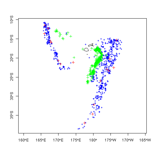
# Convert to simple features
quakes_sf <- st_as_sf(quakes_sp_df)
plot(quakes_sp_df[,3],cex=log(quakes_sf$depth/100), pch=21, bg=24, lwd=.4, axes=T)